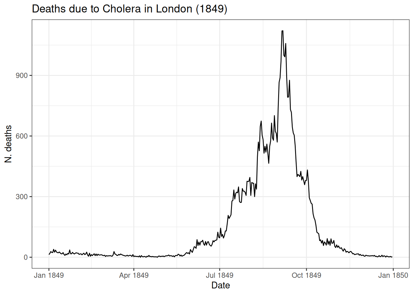
6.3.1 Example: Cholera

Deaths due to cholera over 12 months in 1849 (from the {HistData} package):

library(tidyverse)
library(HistData)

cholera <- HistData::CholeraDeaths1849 %>%
  filter(cause_of_death == "Cholera") %>%
  select(date, deaths)

cholera %>% head()

## # A tibble: 6 × 2
##   date       deaths
##   <date>      <dbl>
## 1 1849-01-01     13
## 2 1849-01-02     19
## 3 1849-01-03     28
## 4 1849-01-04     24
## 5 1849-01-05     23
## 6 1849-01-06     39

Response ($y$) = deaths.

Predictor ($x$) = date.

How to model this?

Review the relationship between response and predictor:

• Equation of a line: $y = \beta_0 + \beta_1x$ or ($y=mx+b$)

• $\beta_0$ - intercept, or value of $y$ when $x = 0$

• $\beta_1$ - average change in $y$ for each unit increase in $x$

• $x$ - value of the predictor

Often there are multiple predictors, adding more complexity to a model.

Modelling estimates these values

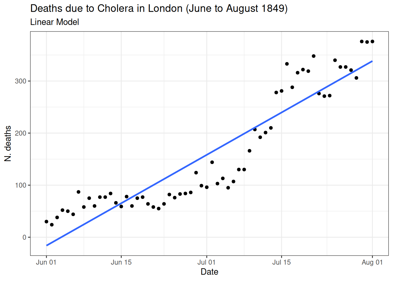
Linear models and Locally estimated scatter plot smoothing (LOESS)

Linear model

• Assumes linear relationship.

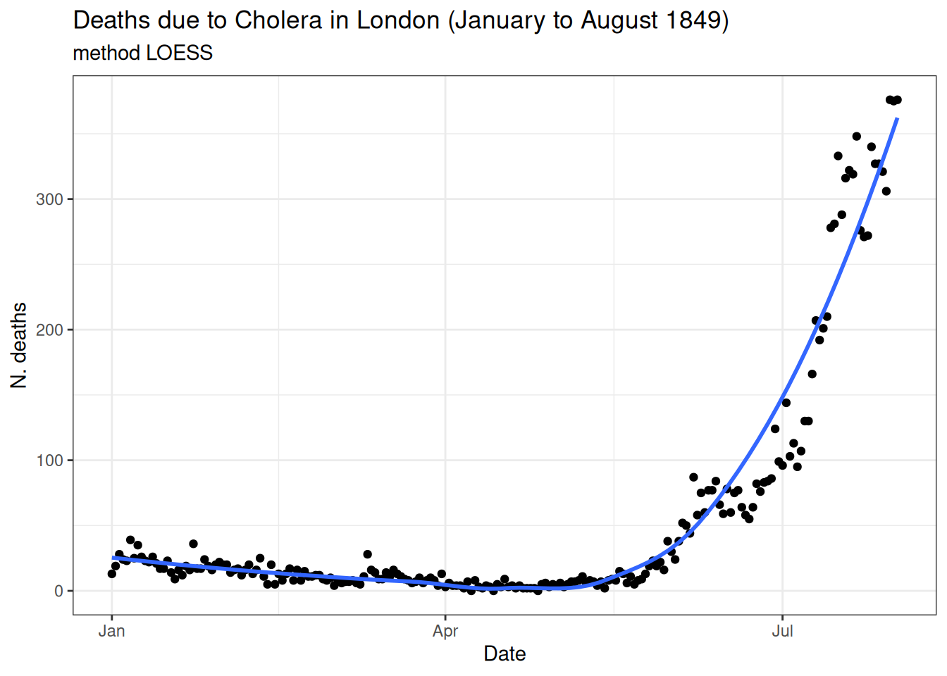
Locally estimated scatter plot smoothing (LOESS)

• No underlying assumptions made about the structure of the data.

Comparing linear and non-linear models

Plotting a linear model against a generalised additive model (GAM):

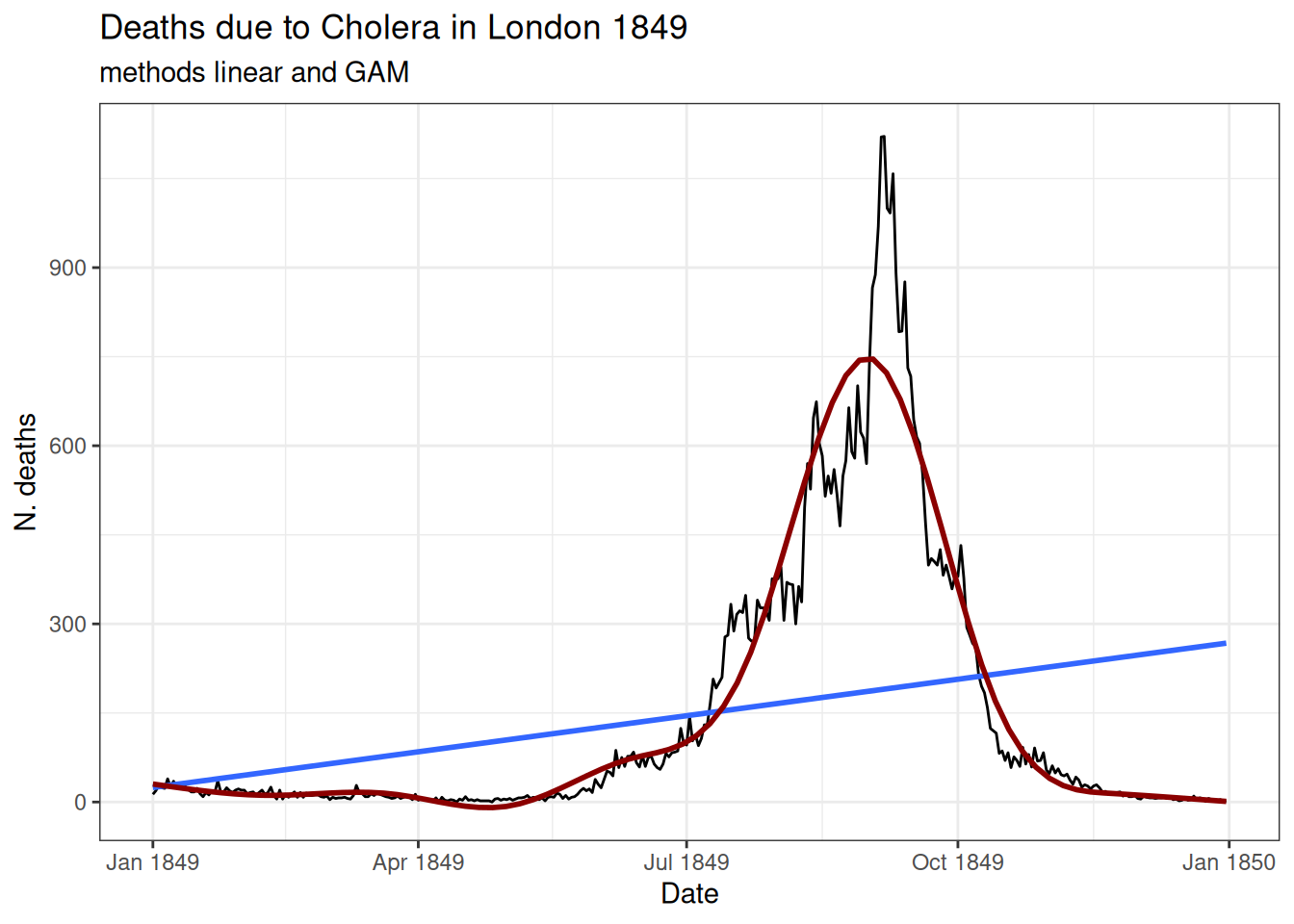
GAM - Generalised Additive Model

What are they?

• Flexible extensions of linear models.
• Useful for modelling complex relationships between response ($y$) and predictor(s) ($x_1,...x_n$).

$g(\mu) = \beta_0 + f(x)$

• Predictors are transformed through each function $x \sim f(x)$.
• Link function $g(\mu)$ is chosen based on response distribution.

How to do this in R?

# Load the mgcv package
library(mgcv)

# Use the days instead of the full date
cholera$days <- row_number(cholera)

# Look at the first six rows
head(cholera)

## # A tibble: 6 × 3
##   date       deaths  days
##   <date>      <dbl> <int>
## 1 1849-01-01     13     1
## 2 1849-01-02     19     2
## 3 1849-01-03     28     3
## 4 1849-01-04     24     4
## 5 1849-01-05     23     5
## 6 1849-01-06     39     6

# Fit a GAM using the gam() function
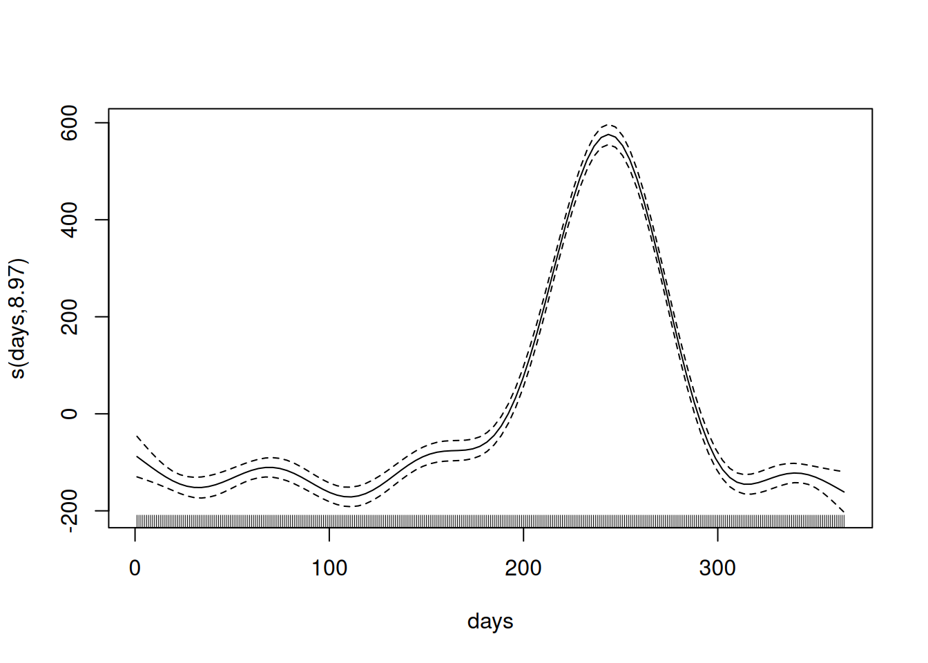
gam_model <- gam(deaths ~ s(days), data = cholera)

# Print the summary of the GAM model
summary(gam_model)

## 
## Family: gaussian 
## Link function: identity 
## 
## Formula:
## deaths ~ s(days)
## 
## Parametric coefficients:
##             Estimate Std. Error t value Pr(>|t|)    
## (Intercept)  146.008      3.583   40.74   <2e-16 ***
## ---
## Signif. codes:  0 '***' 0.001 '**' 0.01 '*' 0.05 '.' 0.1 ' ' 1
## 
## Approximate significance of smooth terms:
##           edf Ref.df     F p-value    
## s(days) 8.969      9 431.4  <2e-16 ***
## ---
## Signif. codes:  0 '***' 0.001 '**' 0.01 '*' 0.05 '.' 0.1 ' ' 1
## 
## R-sq.(adj) =  0.914   Deviance explained = 91.6%
## GCV = 4818.7  Scale est. = 4687      n = 365

Key points:

• Intercept is modelled as a parametric term.
• Days is a smooth term: s(days).
• Effective degrees of freedom (EDF) is ~9, indicating a wiggly (non-linear) relationship to deaths.
• Adjusted R-squared value indicates the model explains approx. 91.4% of variance in $y$.
• Deviance value of 91.6% indicates a good fit.

plot(gam_model)

However, the model is very simple with only one predictor. In reality there are likely to be many other factors that influence number of deaths.