4.4 Prototype

The first version of the app is a dashboard, where the user can choose a product and get the tables and the plot we have seen in the previous chapter.

Code of the ui:

ui <- fluidPage(
  # choose product
  fluidRow(
    column(
      width = 6,
      selectInput(inputId = "code", label = "Product", choices = prod_codes)
    )
  ),
  # display tables
  fluidRow(
    column(width = 4, tableOutput(outputId = "diag")),
    column(width = 4, tableOutput(outputId = "body_part")),
    column(width = 4, tableOutput(outputId = "location"))
  ),
  # display plot
  fluidRow(
    column(width = 12, plotOutput(outputId = "age_sex"))
  )
)

Code of the server:

server <- function(input, output, session) {
  # reactive for filtered data frame
  selected <- reactive(
    injuries %>%
      filter(prod_code == input$code)
  )
  
  # render diagnosis table
  output$diag <- renderTable(
    selected() %>%
      count(diag, wt = weight, sort = TRUE)
  )
  
  # render body part table
  output$body_part <- renderTable(
    selected() %>%
      count(body_part, wt = weight, sort = TRUE)
  )
  
  # render location table
  output$location <- renderTable(
    selected() %>%
      count(location, wt = weight, sort = TRUE)
  )
  
  # reactive for plot data
  summary <- reactive(
    selected() %>%
      count(age, sex, wt = weight) %>%
      left_join(y = population, by = c("age", "sex")) %>%
      mutate(rate = n / population * 1e4)
  )
  
  # render plot
  output$age_sex <- renderPlot(
    expr = {
      summary() %>%
        ggplot(mapping = aes(x = age, y = n, colour = sex)) +
        geom_line() +
        labs(y = "Estimated number of injuries")
    },
    res = 96
  )
}

Note: The reactive for plot data is only used once. You could also compute the dataframe when rendering the plot, but it is good practise to seperate computing and plotting. It’s easier to understand and generalise.

This prototype is available at https://hadley.shinyapps.io/ms-prototype/.

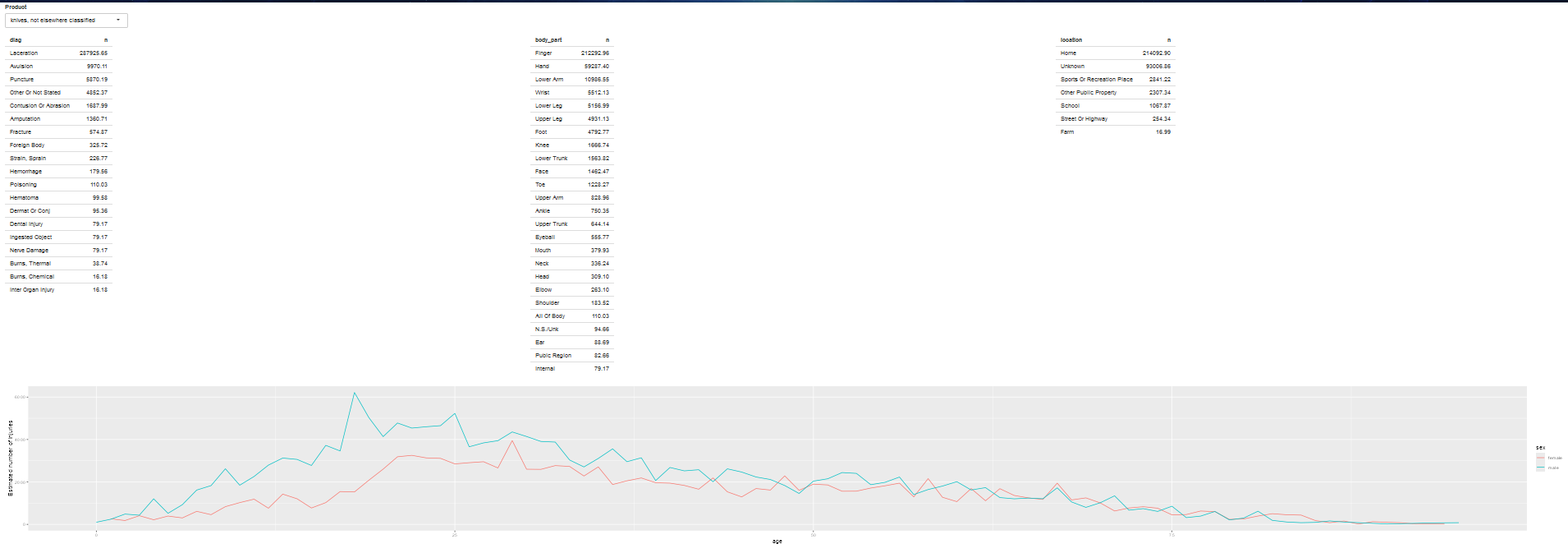
prototype of the app