4.3 Exploration

As motivation for the app we want to build, we’re going to explore the data.

Let’s have a look at accidents related to toilets:

# product code for toilets is 649
selected <- injuries %>% filter(prod_code == 649)

# nrow(selected): 2993

We’re interested in how many accidents related to toilets we see for different locations, body parts and diagnosis.

selected %>%
  count(location, wt = weight, sort = TRUE)

## # A tibble: 6 × 2
##   location                         n
##   <chr>                        <dbl>
## 1 Home                       99603. 
## 2 Other Public Property      18663. 
## 3 Unknown                    16267. 
## 4 School                       659. 
## 5 Street Or Highway             16.2
## 6 Sports Or Recreation Place    14.8

selected %>%
  count(body_part, wt = weight, sort = TRUE)

## # A tibble: 24 × 2
##    body_part        n
##    <chr>        <dbl>
##  1 Head        31370.
##  2 Lower Trunk 26855.
##  3 Face        13016.
##  4 Upper Trunk 12508.
##  5 Knee         6968.
##  6 N.S./Unk     6741.
##  7 Lower Leg    5087.
##  8 Shoulder     3590.
##  9 All Of Body  3438.
## 10 Ankle        3315.
## # ℹ 14 more rows

selected %>%
  count(diag, wt = weight, sort = TRUE)

## # A tibble: 20 × 2
##    diag                        n
##    <chr>                   <dbl>
##  1 Other Or Not Stated   32897. 
##  2 Contusion Or Abrasion 22493. 
##  3 Inter Organ Injury    21525. 
##  4 Fracture              21497. 
##  5 Laceration            18734. 
##  6 Strain, Sprain         7609. 
##  7 Dislocation            2713. 
##  8 Hematoma               2386. 
##  9 Avulsion               1778. 
## 10 Nerve Damage           1091. 
## 11 Poisoning               928. 
## 12 Concussion              822. 
## 13 Dental Injury           199. 
## 14 Hemorrhage              167. 
## 15 Crushing                114. 
## 16 Dermat Or Conj           84.2
## 17 Burns, Not Spec          67.2
## 18 Puncture                 67.2
## 19 Burns, Thermal           34.0
## 20 Burns, Scald             17.0

Weights?

• The NEISS data dictionary calls this column “Statistical Weight for National Estimates”
• perhaps a form of propensity weighting

Next we’ll we create a plot for the number of accidents for different age and sex:

summary <- selected %>%
  count(age, sex, wt = weight) %>% 
  left_join(y = population, by = c("age", "sex")) %>% 
  mutate(rate = n / population * 1e4)

summary %>%
  ggplot(mapping = aes(x = age, y = rate, color = sex)) +
  geom_line(na.rm = TRUE) +
  labs(y = "Injuries per 10,000 people")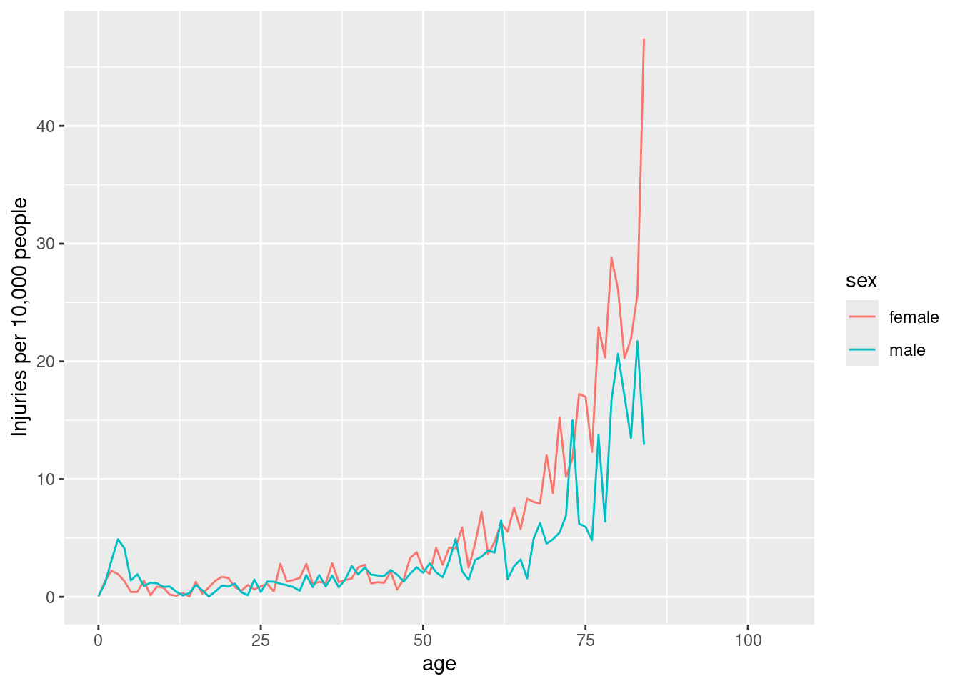

4.3.1 Facet Wrap

Let us briefly look at all of the injury types in the data set.

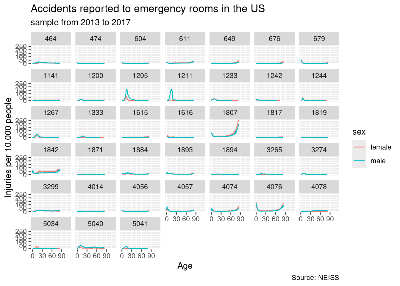
Image code

injuries |>
  group_by(prod_code) |>
  count(age, sex, wt = weight) |> 
  left_join(y = population, by = c("age", "sex")) |>
  mutate(rate = n / population * 1e4) |>
  ggplot(mapping = aes(x = age, y = rate, color = sex)) +
  geom_line(na.rm = TRUE) +
  facet_wrap(vars(prod_code)) +
  labs(title = "Accidents reported to emergency rooms in the US",
       subtitle = "sample from 2013 to 2017",
       caption = "Source: NEISS",
       x = "Age",
       y = "Injuries per 10,000 people")

The goal is to build an app, which outputs the tables and the plot for different products, which the user selects.