12.3 Data-masking

Data-masking functions allow you to use variables in the “current” data frame without any extra syntax. It’s used in many dplyr functions like arrange(), filter(), group_by(), mutate(), and summarise(), and in ggplot2’s aes(). Data-masking is useful because it lets you use data-variables without any additional syntax.

12.3.1 Getting Started

This is a call to filter() which uses a data-variable (carat) and an env-variable (min):

min <- 1
diamonds %>% filter(carat > min)

## # A tibble: 17,502 × 10
##    carat cut       color clarity depth table price     x     y     z
##    <dbl> <ord>     <ord> <ord>   <dbl> <dbl> <int> <dbl> <dbl> <dbl>
##  1  1.17 Very Good J     I1       60.2    61  2774  6.83  6.9   4.13
##  2  1.01 Premium   F     I1       61.8    60  2781  6.39  6.36  3.94
##  3  1.01 Fair      E     I1       64.5    58  2788  6.29  6.21  4.03
##  4  1.01 Premium   H     SI2      62.7    59  2788  6.31  6.22  3.93
##  5  1.05 Very Good J     SI2      63.2    56  2789  6.49  6.45  4.09
##  6  1.05 Fair      J     SI2      65.8    59  2789  6.41  6.27  4.18
##  7  1.01 Fair      E     SI2      67.4    60  2797  6.19  6.05  4.13
##  8  1.04 Premium   G     I1       62.2    58  2801  6.46  6.41  4   
##  9  1.2  Fair      F     I1       64.6    56  2809  6.73  6.66  4.33
## 10  1.02 Premium   G     I1       60.3    58  2815  6.55  6.5   3.94
## # ℹ 17,492 more rows

This is its base R equivalent:

diamonds[diamonds$carat > min, ]

## # A tibble: 17,502 × 10
##    carat cut       color clarity depth table price     x     y     z
##    <dbl> <ord>     <ord> <ord>   <dbl> <dbl> <int> <dbl> <dbl> <dbl>
##  1  1.17 Very Good J     I1       60.2    61  2774  6.83  6.9   4.13
##  2  1.01 Premium   F     I1       61.8    60  2781  6.39  6.36  3.94
##  3  1.01 Fair      E     I1       64.5    58  2788  6.29  6.21  4.03
##  4  1.01 Premium   H     SI2      62.7    59  2788  6.31  6.22  3.93
##  5  1.05 Very Good J     SI2      63.2    56  2789  6.49  6.45  4.09
##  6  1.05 Fair      J     SI2      65.8    59  2789  6.41  6.27  4.18
##  7  1.01 Fair      E     SI2      67.4    60  2797  6.19  6.05  4.13
##  8  1.04 Premium   G     I1       62.2    58  2801  6.46  6.41  4   
##  9  1.2  Fair      F     I1       64.6    56  2809  6.73  6.66  4.33
## 10  1.02 Premium   G     I1       60.3    58  2815  6.55  6.5   3.94
## # ℹ 17,492 more rows

Base R functions refer to data-variables with $, and you often have to repeat the name of the data frame multiple times, making it clear what is a data-variable and what is an env-variable.

It also makes it straightforward to use indirection because you can store the name of the data-variable in an env-variable, and then switch from $ to [[:

var <- "carat"
diamonds[diamonds[[var]] > min, ]

## # A tibble: 17,502 × 10
##    carat cut       color clarity depth table price     x     y     z
##    <dbl> <ord>     <ord> <ord>   <dbl> <dbl> <int> <dbl> <dbl> <dbl>
##  1  1.17 Very Good J     I1       60.2    61  2774  6.83  6.9   4.13
##  2  1.01 Premium   F     I1       61.8    60  2781  6.39  6.36  3.94
##  3  1.01 Fair      E     I1       64.5    58  2788  6.29  6.21  4.03
##  4  1.01 Premium   H     SI2      62.7    59  2788  6.31  6.22  3.93
##  5  1.05 Very Good J     SI2      63.2    56  2789  6.49  6.45  4.09
##  6  1.05 Fair      J     SI2      65.8    59  2789  6.41  6.27  4.18
##  7  1.01 Fair      E     SI2      67.4    60  2797  6.19  6.05  4.13
##  8  1.04 Premium   G     I1       62.2    58  2801  6.46  6.41  4   
##  9  1.2  Fair      F     I1       64.6    56  2809  6.73  6.66  4.33
## 10  1.02 Premium   G     I1       60.3    58  2815  6.55  6.5   3.94
## # ℹ 17,492 more rows

We can achieve the same result with tidy evaluation by somehow adding $ back into the picture while data-masking functions by using .data or .env to be explicit about whether you’re talking about a data-variable or an env-variable:

diamonds %>% filter(.data$carat > .env$min)

diamonds %>% filter(.data[[var]] > .env$min)

num_vars <- c("carat", "depth", "table", "price", "x", "y", "z")
ui <- fluidPage(
  selectInput("var", "Variable", choices = num_vars),
  numericInput("min", "Minimum", value = 1),
  tableOutput("output")
)
server <- function(input, output, session) {
  data <- reactive(diamonds %>% filter(.data[[input$var]] > .env$input$min))
  output$output <- renderTable(head(data()))
}

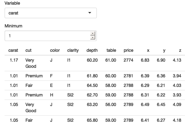
The app works now that we’ve been explicit about .data and .env and [[ vs $. See live at https://hadley.shinyapps.io/ms-tidied-up.

12.3.2 Example: ggplot2

Here we apply this idea to a dynamic plot where we allow the user to create a scatterplot by selecting the variables to appear on the x and y axes. ggforce::position_auto() was used so that geom_point() works regardless of whether the x and y variables are continuous or discrete.

ui <- fluidPage(
  selectInput("x", "X variable", choices = names(iris)),
  selectInput("y", "Y variable", choices = names(iris)),
  plotOutput("plot")
)
server <- function(input, output, session) {
  output$plot <- renderPlot({
    ggplot(iris, aes(.data[[input$x]], .data[[input$y]])) +
      geom_point(position = ggforce::position_auto())
  }, res = 96)
}

Alternatively, we could allow the user to pick the geom. The following app uses a switch() statement to generate a reactive geom that is later added to the plot.

ui <- fluidPage(
  selectInput("x", "X variable", choices = names(iris)),
  selectInput("y", "Y variable", choices = names(iris)),
  selectInput("geom", "geom", c("point", "smooth", "jitter")),
  plotOutput("plot")
)
server <- function(input, output, session) {
  plot_geom <- reactive({
    switch(input$geom,
      point = geom_point(),
      smooth = geom_smooth(se = FALSE),
      jitter = geom_jitter()
    )
  })
  
  output$plot <- renderPlot({
    ggplot(iris, aes(.data[[input$x]], .data[[input$y]])) +
      plot_geom()
  }, res = 96)
}

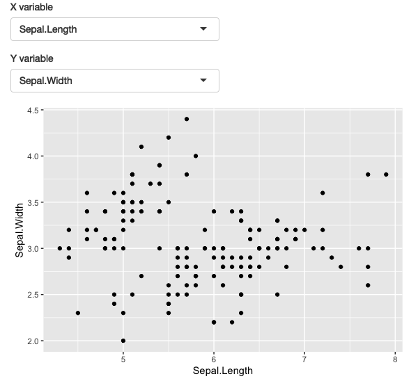
This app allows you to select which variables are plotted on the x and y axes. See live at https://hadley.shinyapps.io/ms-ggplot2.

One of the challenges of programming with user selected variables is that your code has to become more complicated to handle all the cases the user might generate.

12.3.3 Example: dplyr

The same technique also works for dplyr. The following app extends the previous simple example to allow you to choose a variable to filter, a minimum value to select, and a variable to sort by.

ui <- fluidPage(
  selectInput("var", "Select variable", choices = names(mtcars)),
  sliderInput("min", "Minimum value", 0, min = 0, max = 100),
  selectInput("sort", "Sort by", choices = names(mtcars)),
  tableOutput("data")
)
server <- function(input, output, session) {
  observeEvent(input$var, {
    rng <- range(mtcars[[input$var]])
    updateSliderInput(
      session, "min", 
      value = rng[[1]], 
      min = rng[[1]], 
      max = rng[[2]]
    )
  })
  
  output$data <- renderTable({
    mtcars %>% 
      filter(.data[[input$var]] > input$min) %>% 
      arrange(.data[[input$sort]])
  })
}

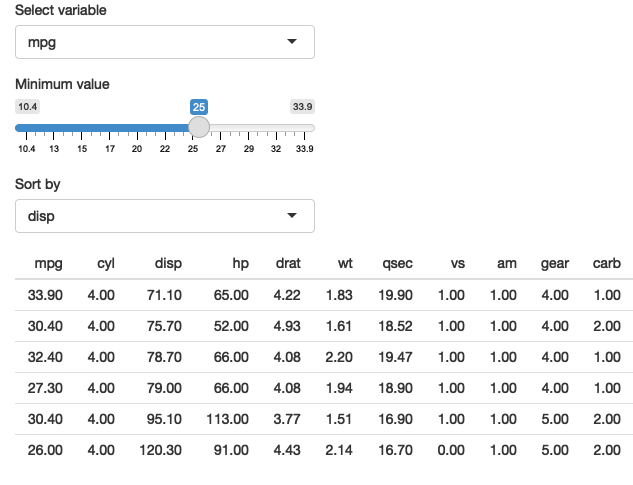
This app that allows you to pick a variable to threshold, and choose how to sort the results. See live at https://hadley.shinyapps.io/ms-dplyr.

Most other problems can be solved by combining .data with your existing programming skills. For example, what if you wanted to conditionally sort in either ascending or descending order?

ui <- fluidPage(
  selectInput("var", "Sort by", choices = names(mtcars)),
  checkboxInput("desc", "Descending order?"),
  tableOutput("data")
)
server <- function(input, output, session) {
  sorted <- reactive({
    if (input$desc) {
      arrange(mtcars, desc(.data[[input$var]]))
    } else {
      arrange(mtcars, .data[[input$var]])
    }
  })
  output$data <- renderTable(sorted())
}

12.3.4 User supplied data

This app allows the user to upload a tsv file, then select a variable and filter by it. It will work for the vast majority of inputs that you might try it with.

ui <- fluidPage(
  fileInput("data", "dataset", accept = ".tsv"),
  selectInput("var", "var", character()),
  numericInput("min", "min", 1, min = 0, step = 1),
  tableOutput("output")
)
server <- function(input, output, session) {
  data <- reactive({
    req(input$data)
    vroom::vroom(input$data$datapath)
  })
  observeEvent(data(), {
    updateSelectInput(session, "var", choices = names(data()))
  })
  observeEvent(input$var, {
    val <- data()[[input$var]]
    updateNumericInput(session, "min", value = min(val))
  })
  
  output$output <- renderTable({
    req(input$var)
    
    data() %>% 
      filter(.data[[input$var]] > input$min) %>% 
      arrange(.data[[input$var]]) %>% 
      head(10)
  })
}

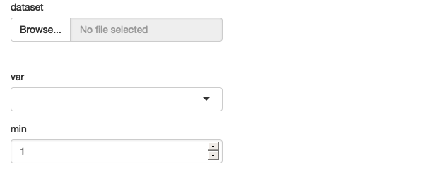
An app that filter users supplied data, with a surprising failure mode See live at https://hadley.shinyapps.io/ms-user-supplied.

It’ll work with the vast majority of data frames. However, if the data frame contains a variable called input, we get an error message because filter() is attempting to evaluate df$input$min:

df <- data.frame(x = 1, y = 2)
input <- list(var = "x", min = 0)

df %>% filter(.data[[input$var]] > input$min)

df <- data.frame(x = 1, y = 2, input = 3)
df %>% filter(.data[[input$var]] > input$min)

This problem is due to the ambiguity of data-variables and env-variables, and because data-masking prefers to use a data-variable if both are available. We can resolve the problem by using .env to tell filter() only look for min in the env-variables:

df %>% filter(.data[[input$var]] > .env$input$min)

You only need to worry about this problem when working with user supplied data; when working with your own data, you can ensure the names of your data-variables don’t clash with the names of your env-variables.

12.3.5 Why not use base R?

You might wonder if you’re better off without filter(), and if instead you should use the equivalent base R code:

df[df[[input$var]] > input$min, ]

That’s a totally legitimate position, as long as you’re aware of the work that filter() does for you so you can generate the equivalent base R code. In this case:

• You’ll need drop = FALSE if df only contains a single column (otherwise you’ll get a vector instead of a data frame).

• You’ll need to use which() or similar to drop any missing values.

• You can’t do group-wise filtering (e.g. df %>% group_by(g) %>% filter(n() == 1)).

In general, if you’re using dplyr for very simple cases, you might find it easier to use base R functions that don’t use data-masking. However, in my opinion, one of the advantages of the tidyverse is the careful thought that has been applied to edge cases so that functions work more consistently.