4.5 Polish tables
Now we’re going to improve the app step-by-step.
The prototype version of the app has very long tables. To make it a little clearer we only want to show the top 5 and lump together all other categories in every table.
As an example the diagnosis table for all products would look like this:
injuries %>%
  mutate(diag = fct_lump(fct_infreq(diag), n = 5)) %>%
  group_by(diag) %>%
  summarise(n = as.integer(sum(weight)))
## # A tibble: 6 × 2
## diag n
## <fct> <int>
## 1 Other Or Not Stated 1806436
## 2 Fracture 1558961
## 3 Laceration 1432407
## 4 Strain, Sprain 1432556
## 5 Contusion Or Abrasion 1451987
## 6 Other 19291474.5.1 Exercise 4.8.2
- What happens if you flip
fct_infreq()andfct_lump()in the code that reduces the summary tables?
Answer
injuries %>%
  mutate(diag = fct_infreq(fct_lump(diag, n = 5))) %>%
  group_by(diag) %>%
  summarise(n = as.integer(sum(weight)))
## # A tibble: 6 × 2
## diag n
## <fct> <int>
## 1 Other 1929147
## 2 Other Or Not Stated 1806436
## 3 Fracture 1558961
## 4 Laceration 1432407
## 5 Strain, Sprain 1432556
## 6 Contusion Or Abrasion 1451987This order lumped the rarer conditions into “Other” and then did the sorting. However, since “Other” was the most frequent label, fct_infreq() then put “Other” at the top, which is less desirable.
4.5.2 Hadley’s Fix
Hadley’s Code
count_top <- function(df, var, n = 5) {
  df %>%
    mutate({{ var }} := fct_lump(fct_infreq({{ var }}), n = n)) %>%
    group_by({{ var }}) %>%
    summarise(n = as.integer(sum(weight)))
}

output$diag <- renderTable(count_top(selected(), diag), width = "100%")
output$body_part <- renderTable(count_top(selected(), body_part), width = "100%")
output$location <- renderTable(count_top(selected(), location), width = "100%")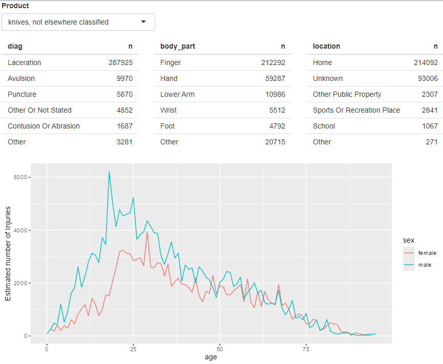
polished tables