4.6 Visualizations for Categorical Data: Exploring the OKCupid dataset

OkCupid is an online dating site that serves international users. Kim and Escobedo-Land (2015) describe a data set where over 50,000 profiles from the San Francisco area.

load(url("https://github.com/topepo/FES/blob/master/Data_Sets/OkCupid/okc.RData?raw=true"))

First look at the dataset

# bind 'okc_test'
okc <- okc_train %>%
  bind_rows(okc_test)

Skim okc

skimr::skim(okc) %>% 
  knitr::kable()

skim_type	skim_variable	n_missing	complete_rate	factor.ordered	factor.n_unique	factor.top_counts	numeric.mean	numeric.sd	numeric.p0	numeric.p25	numeric.p50	numeric.p75	numeric.p100	numeric.hist
factor	diet	0	1	FALSE	19	die: 19691, mos: 15229, any: 5440, str: 4583	NA	NA	NA	NA	NA	NA	NA	NA
factor	drinks	0	1	FALSE	7	soc: 36756, rar: 5328, oft: 4531, not: 2868	NA	NA	NA	NA	NA	NA	NA	NA
factor	drugs	0	1	FALSE	4	nev: 32805, dru: 11758, som: 6818, oft: 366	NA	NA	NA	NA	NA	NA	NA	NA
factor	education	0	1	FALSE	33	gra: 21423, gra: 8151, wor: 5193, ed_: 3572	NA	NA	NA	NA	NA	NA	NA	NA
factor	income	0	1	FALSE	13	mis: 40584, inc: 2876, inc: 1572, inc: 1080	NA	NA	NA	NA	NA	NA	NA	NA
factor	offspring	0	1	FALSE	16	kid: 29360, doe: 6744, doe: 3653, doe: 3322	NA	NA	NA	NA	NA	NA	NA	NA
factor	pets	0	1	FALSE	16	pet: 15181, lik: 13642, lik: 6534, lik: 3988	NA	NA	NA	NA	NA	NA	NA	NA
factor	religion	0	1	FALSE	10	rel: 15333, agn: 8043, oth: 7231, ath: 6316	NA	NA	NA	NA	NA	NA	NA	NA
factor	sign	0	1	FALSE	13	sig: 7818, leo: 3922, gem: 3911, can: 3784	NA	NA	NA	NA	NA	NA	NA	NA
factor	smokes	0	1	FALSE	6	no: 38941, smo: 3619, som: 3268, whe: 2688	NA	NA	NA	NA	NA	NA	NA	NA
factor	status	0	1	FALSE	5	sin: 48032, see: 1814, ava: 1624, mar: 269	NA	NA	NA	NA	NA	NA	NA	NA
factor	where_state	0	1	FALSE	36	cal: 51672, new: 15, ill: 6, mas: 4	NA	NA	NA	NA	NA	NA	NA	NA
factor	where_town	0	1	FALSE	51	san: 26683, oak: 6214, ber: 3616, san: 1168	NA	NA	NA	NA	NA	NA	NA	NA
factor	religion_modifer	0	1	FALSE	5	rel: 25718, but: 11469, and: 8309, and: 4221	NA	NA	NA	NA	NA	NA	NA	NA
factor	sign_modifer	0	1	FALSE	4	sig: 17909, and: 17709, but: 15511, and: 618	NA	NA	NA	NA	NA	NA	NA	NA
factor	Class	0	1	FALSE	2	oth: 42190, ste: 9557	NA	NA	NA	NA	NA	NA	NA	NA
numeric	age	0	1	NA	NA	NA	3.255509e+01	9.518919e+00	18	26.000000	30.000000	37.000000	109.000000	▇▂▁▁▁
numeric	height	0	1	NA	NA	NA	6.833121e+01	3.979818e+00	1	66.000000	68.000000	71.000000	95.000000	▁▁▁▇▁
numeric	last_online	0	1	NA	NA	NA	3.916536e+01	7.625808e+01	0	1.000000	4.000000	30.000000	370.000000	▇▁▁▁▁
numeric	cpp	0	1	NA	NA	NA	2.898700e-03	5.376220e-02	0	0.000000	0.000000	0.000000	1.000000	▇▁▁▁▁
numeric	cpp_fluently	0	1	NA	NA	NA	1.252250e-02	1.112020e-01	0	0.000000	0.000000	0.000000	1.000000	▇▁▁▁▁
numeric	cpp_okay	0	1	NA	NA	NA	9.855600e-03	9.878610e-02	0	0.000000	0.000000	0.000000	1.000000	▇▁▁▁▁
numeric	cpp_poorly	0	1	NA	NA	NA	7.382100e-03	8.560210e-02	0	0.000000	0.000000	0.000000	1.000000	▇▁▁▁▁
numeric	lisp	0	1	NA	NA	NA	5.991000e-04	2.446880e-02	0	0.000000	0.000000	0.000000	1.000000	▇▁▁▁▁
numeric	lisp_fluently	0	1	NA	NA	NA	1.488000e-03	3.854640e-02	0	0.000000	0.000000	0.000000	1.000000	▇▁▁▁▁
numeric	lisp_okay	0	1	NA	NA	NA	2.319000e-03	4.810030e-02	0	0.000000	0.000000	0.000000	1.000000	▇▁▁▁▁
numeric	lisp_poorly	0	1	NA	NA	NA	2.280300e-03	4.769870e-02	0	0.000000	0.000000	0.000000	1.000000	▇▁▁▁▁
numeric	asian	0	1	NA	NA	NA	1.371094e-01	3.439661e-01	0	0.000000	0.000000	0.000000	1.000000	▇▁▁▁▁
numeric	black	0	1	NA	NA	NA	5.637040e-02	2.306379e-01	0	0.000000	0.000000	0.000000	1.000000	▇▁▁▁▁
numeric	hispanic_latin	0	1	NA	NA	NA	8.937720e-02	2.852901e-01	0	0.000000	0.000000	0.000000	1.000000	▇▁▁▁▁
numeric	indian	0	1	NA	NA	NA	2.467780e-02	1.551426e-01	0	0.000000	0.000000	0.000000	1.000000	▇▁▁▁▁
numeric	middle_eastern	0	1	NA	NA	NA	1.571110e-02	1.243564e-01	0	0.000000	0.000000	0.000000	1.000000	▇▁▁▁▁
numeric	native_american	0	1	NA	NA	NA	2.125730e-02	1.442422e-01	0	0.000000	0.000000	0.000000	1.000000	▇▁▁▁▁
numeric	other	0	1	NA	NA	NA	6.083440e-02	2.390287e-01	0	0.000000	0.000000	0.000000	1.000000	▇▁▁▁▁
numeric	pacific_islander	0	1	NA	NA	NA	2.475510e-02	1.553793e-01	0	0.000000	0.000000	0.000000	1.000000	▇▁▁▁▁
numeric	white	0	1	NA	NA	NA	6.474578e-01	4.777663e-01	0	0.000000	1.000000	1.000000	1.000000	▅▁▁▁▇
numeric	essay_length	0	1	NA	NA	NA	3.132866e+00	6.777757e-01	0	3.009026	3.269513	3.480438	4.983486	▁▁▂▇▁
numeric	profile	0	1	NA	NA	NA	2.587400e+04	1.493822e+04	1	12937.500000	25874.000000	38810.500000	51747.000000	▇▇▇▇▇

Plot Class

okc %>% 
  ggplot(aes(Class, fill = Class)) + 
  geom_bar() + 
  theme(legend.position = 'none')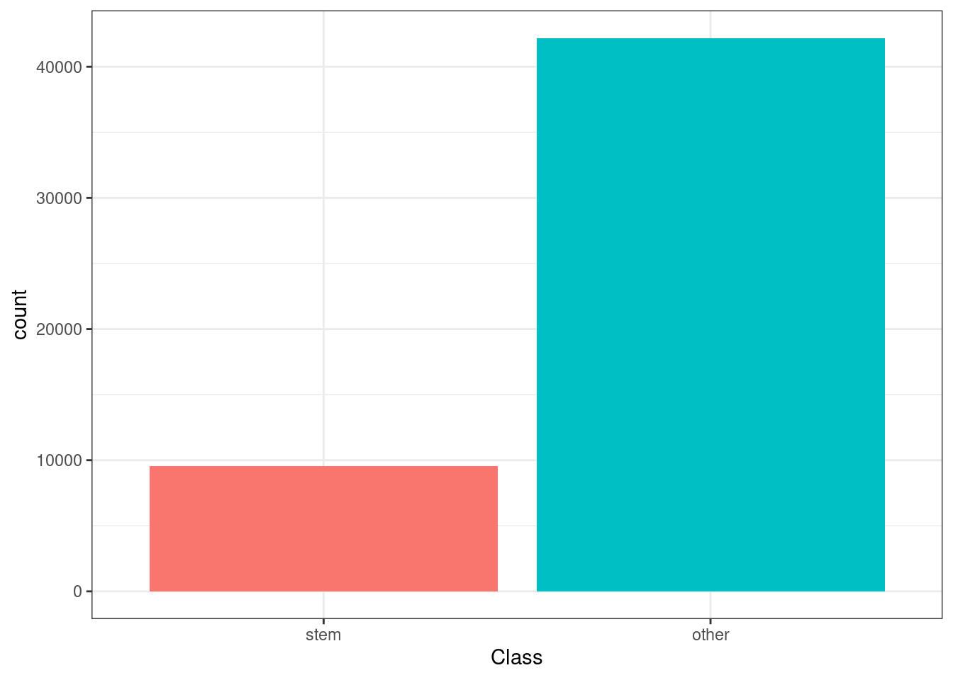

4.6.1 Visualizing Relationships between Outcomes and Predictors

4.6.1.1 Outcome and Categorical Predictor

Let’s plot the frequency of the stated religion, partitioned and color by the outcome (Class).

binom_stats <- function(x, ...) {
  x <- x$Class[!is.na(x$Class)]
  res <- prop.test(x = sum(x == "stem"), n = length(x), ...)
  data.frame(Proportion  = unname(res$estimate), 
             Lower = res$conf.int[1],
             Upper = res$conf.int[2])
}

stem_rate <- mean(okc_train$Class == "stem")

religion_rates <- 
  okc_train %>%
  group_by(religion) %>%
  do(binom_stats(.)) %>%
  arrange(Proportion) %>%
  ungroup() %>%
  mutate(religion = gsub("religion_", "", religion),
         religion = reorder(factor(religion), Proportion))

okc_train <- 
  okc_train %>% 
  mutate(
    religion2 = gsub("religion_", "", as.character(religion)),
    religion2 = factor(religion2, levels = as.character(religion_rates$religion))
  )

bars <- 
  ggplot(okc_train, aes(x = religion2, fill = Class)) +
  geom_bar(position = position_dodge()) + scale_fill_brewer(palette = "Paired") +
  xlab("") +
  theme(legend.position = "top", axis.text = element_text(size = 8)) +
  ggtitle("(a)")

stacked_vars <-
  ggplot(okc_train, aes(x = religion2, fill = Class)) + geom_bar(position = "fill") +
  scale_fill_brewer(palette = "Paired") +
  xlab("") + ylab("Proportion") +
  theme(legend.position = "none", axis.text = element_text(size = 8)) +
  ggtitle("(b)")

ci_plots <- 
  ggplot(religion_rates, aes(x = religion, y = Proportion)) +
  geom_hline(yintercept = stem_rate, col = "red", alpha = .35, lty = 2) + 
  geom_point() +
  geom_errorbar(aes(ymin = Lower, ymax = Upper), width = .1) +
  theme(axis.text = element_text(size = 8)) +
  xlab("") +
  ggtitle("(c)")

bars / stacked_vars / ci_plots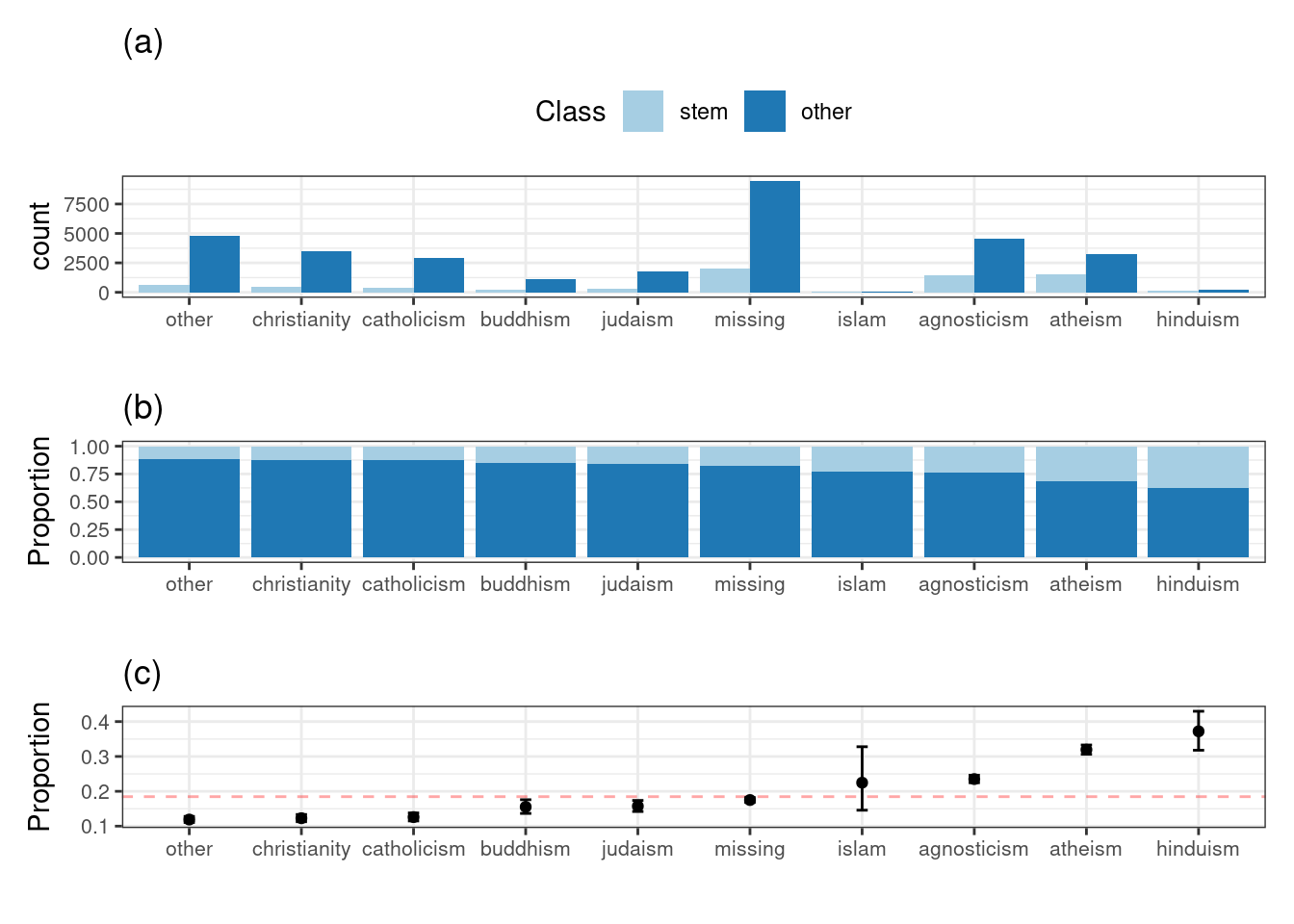

Does religion appear to be related to the outcome? Since there is a gradation of rates of STEM professions between the groups, it would appear so.

4.6.1.2 Outcome and Numerical Predictor

Now, let’s visualize the relationship between a categorical outcome (Class) and a numerical predictor (essay_length).

l10_breaks <- scales::trans_breaks("log10", function(x) 10^x)
l10_labels <- scales::trans_format("log10", scales::math_format(10^.x))

gam_dat <- 
  okc_train %>% 
  dplyr::select(essay_length, Class) %>% 
  arrange(essay_length)

gam_small <- 
  gam_dat %>%
  distinct(essay_length) 

gam_mod <- mgcv::gam(Class ~ s(essay_length), data = gam_dat, family = binomial())

gam_small <- gam_small %>%
  mutate(
    link = -predict(gam_mod, gam_small, type = "link"),
    se = predict(gam_mod, gam_small, type = "link", se.fit = TRUE)$se.fit,
    upper = link + qnorm(.975) * se,
    lower = link - qnorm(.975) * se,
    lower = binomial()$linkinv(lower),
    upper = binomial()$linkinv(upper),
    probability = binomial()$linkinv(link)
  )

brks <- l10_breaks(exp(okc_train$essay_length))

essay_hist <- 
  ggplot(okc_train, aes(x = exp(essay_length))) + 
  geom_histogram(binwidth = .1, col = "#FEB24C", fill = "#FED976") + 
  facet_wrap(~ Class, ncol = 1) + 
  scale_x_log10(breaks = brks, labels = l10_labels) +
  xlab("Essay Character Length") + 
  theme_bw() +
  theme(plot.margin = unit(c(0,1,0,1.2), "cm")) + 
  ggtitle("(a)")

essay_gam <- 
  ggplot(gam_small, aes(x = exp(essay_length))) + 
  geom_line(aes(y = probability)) + 
  geom_ribbon(aes(ymin = lower, ymax = upper), fill = "grey", alpha = .5) + 
  geom_hline(yintercept = stem_rate, col = "red", alpha = .35, lty = 2)  + 
  scale_x_log10(breaks = brks, labels = l10_labels) +
  theme_bw() + 
  xlab("") +
  theme(plot.margin = unit(c(0,1,0,1.2), "cm"))+ 
  ggtitle("(b)")

essay_hist / essay_gam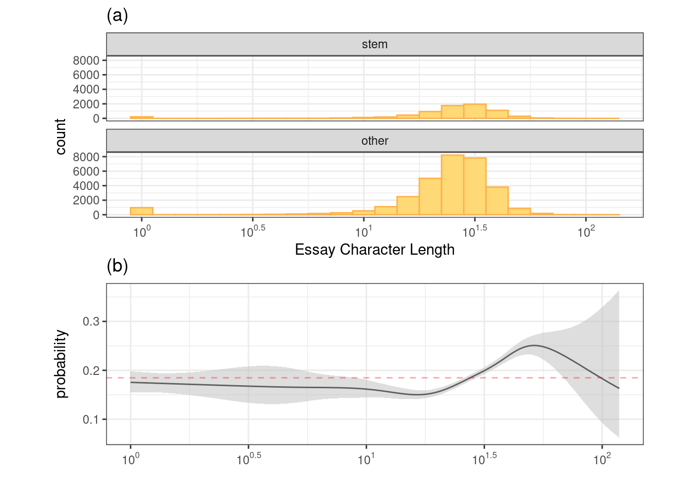

The black line represents the class probability of the logistic regression model and the bands denote 95% confidence intervals around the fit. The horizontal red line indicates the baseline probability of STEM profiles from the training set.

This predictor might be worth including in a model but is unlikely to show a strong effect on its own.

4.6.2 Exploring Relationships Between Categorical Predictors

When considering relationships between categorical data, there are several options. Once a cross-tabulation between variables is created, mosaic plots can once again be used to understand the relationship between variables.

okc_train <- 
  okc_train %>% 
  mutate(
    drugs = factor(as.character(drugs),
                   levels = c("drugs_missing", "never", "sometimes", "often")),
    drinks = factor(as.character(drinks),
                    levels = c("drinks_missing", "not_at_all", "rarely", 
                               "socially", "often", "very_often", "desperately"))
  )

dd_tab <- table(okc_train$drugs, okc_train$drinks, dnn = c("Drugs", "Alcohol"))


# Formatting for slightly better printing
plot_tab <- dd_tab
dimnames(plot_tab)[[1]][1] <- "missing"
dimnames(plot_tab)[[2]] <- gsub("_", " ", dimnames(plot_tab)[[2]])
dimnames(plot_tab)[[2]][1] <- "missing"
dimnames(plot_tab)[[2]][6] <- "often\n"
dimnames(plot_tab)[[2]][6] <- "very often"
dimnames(plot_tab)[[2]][7] <- "\ndesperately"

mosaic(
  t(plot_tab),
  highlighting = TRUE,
  highlighting_fill = rainbow_hcl,
  margins = unit(c(6, 1, 1, 8), "lines"),
  labeling = labeling_border(
    rot_labels = c(90, 0, 0, 0),
    just_labels = c("left", "right",
                    "center",  "right"),
    offset_varnames = unit(c(3, 1, 1, 4), "lines")
  ),
  keep_aspect_ratio = FALSE
)

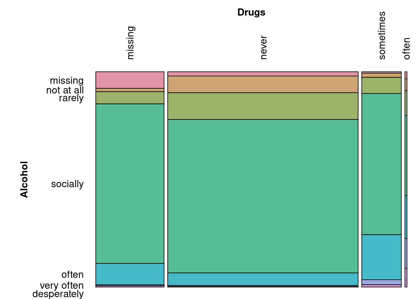
In the cross-tabulation between alcohol and drug use, the χ2 statistic is very large (4043.8) for its degrees of freedom (18) and is associated with a very small p-value (0). This indicates that there is a strong association between these two variables.

ca_obj <- CA(dd_tab, graph = FALSE)

ca_drugs <- as.data.frame(ca_obj$row$coord)
ca_drugs$label <- gsub("_", " ", rownames(ca_drugs))
ca_drugs$Variable <- "Drugs"

ca_drinks <- as.data.frame(ca_obj$col$coord)
ca_drinks$label <- gsub("_", " ", rownames(ca_drinks))
ca_drinks$Variable <- "Alcohol"

ca_rng <- extendrange(c(ca_drinks$`Dim 1`, ca_drinks$`Dim 2`))
ca_x <- paste0("Dimension #1 (",
               round(ca_obj$eig["dim 1", "percentage of variance"], 0),
               "%)")
ca_y <- paste0("Dimension #2 (",
               round(ca_obj$eig["dim 2", "percentage of variance"], 0),
               "%)")

ca_coord <- rbind(ca_drugs, ca_drinks)

ca_plot <-
  ggplot(ca_coord, aes(x = `Dim 1`, y = `Dim 2`, col = Variable)) + 
  geom_vline(xintercept = 0) + 
  geom_hline(yintercept = 0) + 
  geom_text(aes(label = label)) + 
  xlim(ca_rng) + ylim(ca_rng) + 
  xlab(ca_x) + ylab(ca_y) + 
  coord_equal()

ca_plot

## Warning: Removed 1 rows containing missing values (`geom_text()`).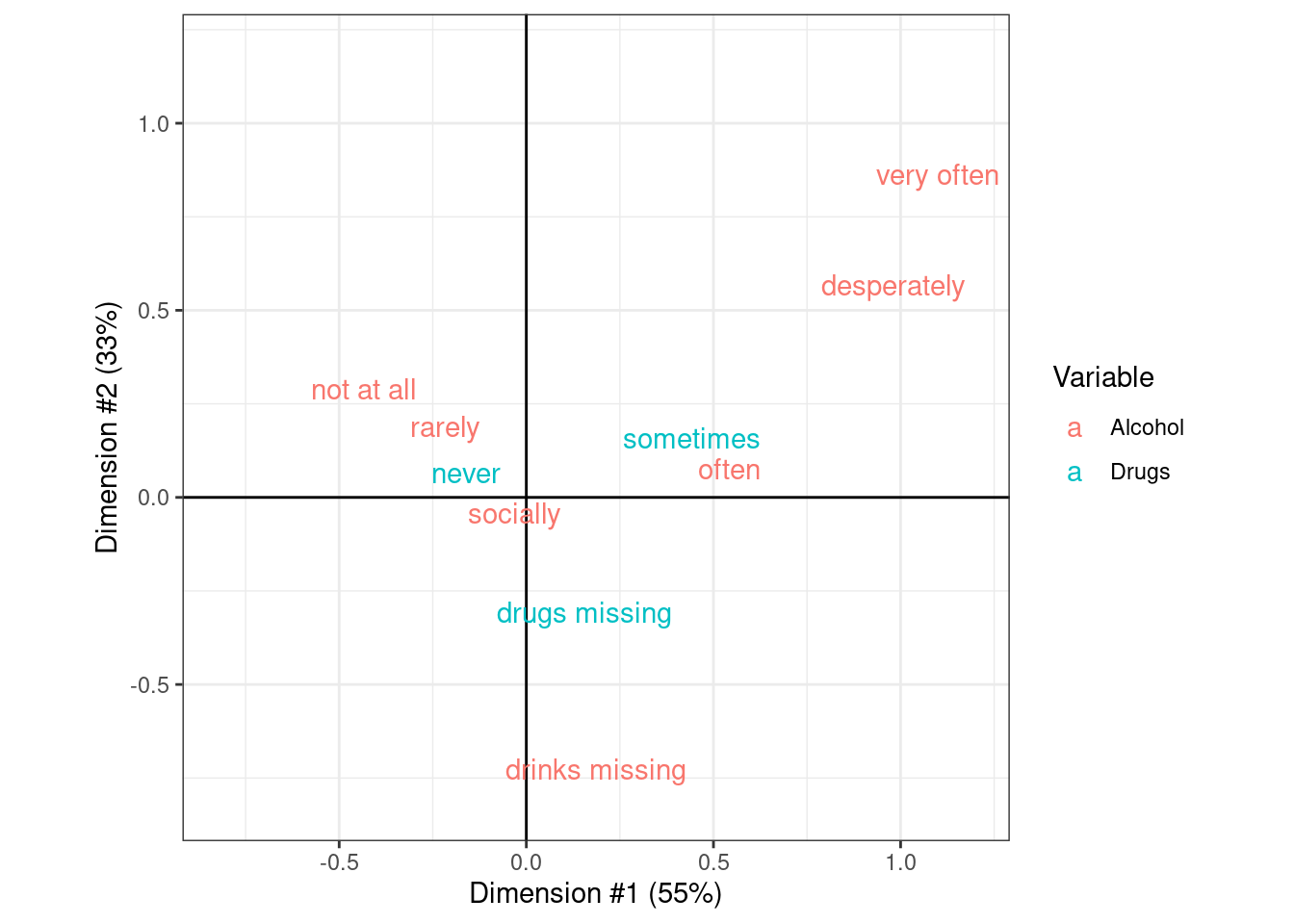

The correspondence analysis principal coordinates for the drug and alcohol data in the OkCupid data.