7.6 Approaches when Complete Enumeration is Practically Impossible
7.6.1 Guiding Principles and Two-stage Modeling
Two-stage Modeling is another approach to use:
- use simple models such as lm or glm then add interaction effects
- use models ready for considering interactions
In the residuals are the predictors missing information.
7.6.1.1 Example
Observed data are \(y\) and \(x_1\), we know nothing about \(x_2\), and so \(x_1*x_2\).
\[y=x_1+x_2+10x_1x_2+\text{error}\]
\[y=\beta_1x_1+x_2+\text{error*}\]
\[\text{error*}=\beta_2x_2+\beta_3x_1x_2+\text{error}\] Random measurement error remains unexplained.
- hierarchy principle: first look at pairwise interactions
- sparsity principle: look for active interactions
- heredity principle: search for interactions among the predictors identified in the first stage
- choose the type of heredity: determine the number of interaction terms
For classification outcome (categorical response) the Pearson residual should be used:
\[\frac{y_i-p_i}{\sqrt{p_i(1-p_i)}}\]
7.6.2 Tree-based Methods
“Tree-based models are usually thought of as pure interaction due to their prediction equation, which can be written as a set of multiplicative statements.”
- tree-based methods uncover potential interactions between variables
- recursive partitioning identifies important interactions among predictors
“In essence, the partitioning aspect of trees impedes their ability to represent smooth, global interactions.”
Moreover, a tree-based model does well at approximating the level of interaction but, it breaks the space into rectangular regions, and needs many regions to capture all possible interactions.
For this reason, ensembles of trees such as bagging (many samples of the original data generated with replacement) and boosting (sequence of trees with restricted depth, improved performance and weighted stats) are better performers.
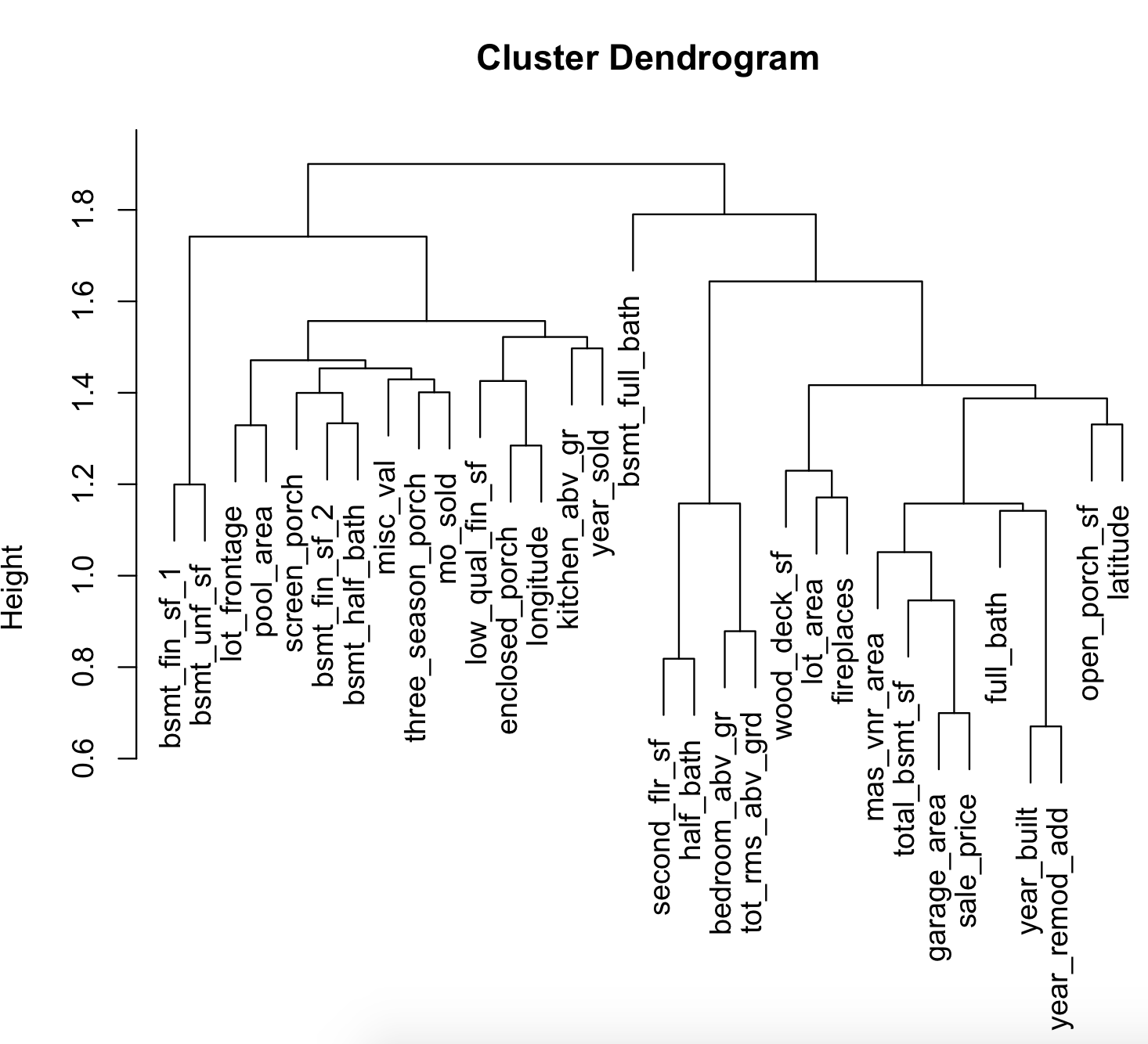
Here is a representation of the clusters for Ames data:
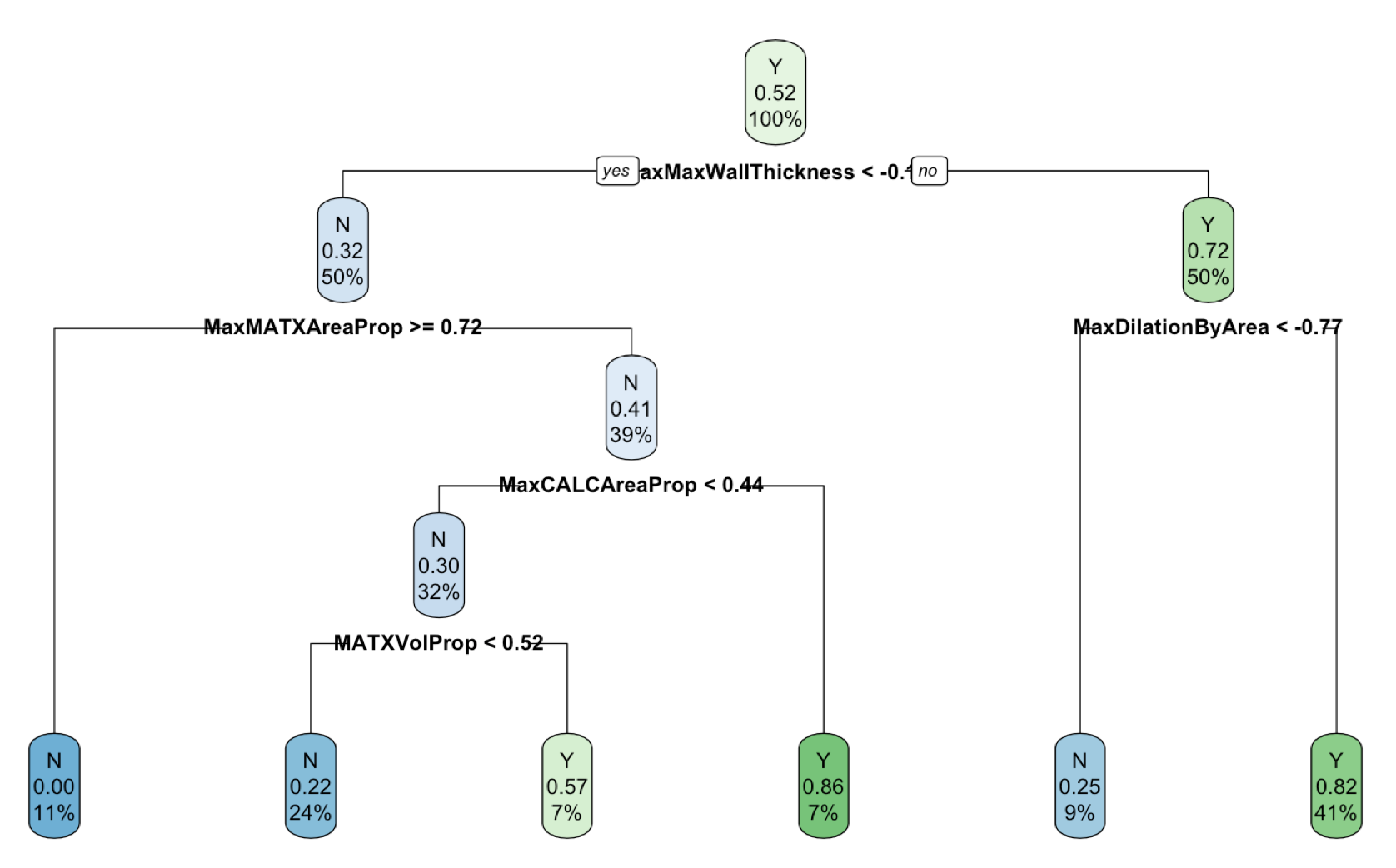
Here is the outcome of a basic decision tree for the Ischemic Stroke data:
see full code in the scripts folder: 6_ames_hclust.R
Tree ensembles are so effective at identifying predictor-response relationships because they are aggregating many trees from slightly different versions of the original data.
An example is Random Forest which is a variation of bagging.
Partial dependency compares the joint effect of two (or more) predictors with the individual effect of each predictor in a model. This comparison is named H statistic, which is 0 if no interaction is found and >0 otherwise.
More about the H statistic can be found in Friedman and Popescu 2008.
see full code in the scripts folder: 7_ames_H_stat.R see the code: Ames trees example with H statistic
Out-of-bag (OOB) samples: Random forest uses bootstrap samples to create many models to be used in the ensemble. Since the bootstrap is being used, each tree has an associated assessment set (historically called the out-of-bag (OOB) samples) that we not used to fit the model.
To be mentioned is this interesting package: pre package
7.6.3 The Feasible Solution Algorithm
A preselction is done before searching for interaction among predictors. When linear and logistic models are used some predictor selection methods are applied:
Forward selection: It starts with no predictors and select the best one, then select the second best and so on…
Backward selection: It starts with all predictors and make a selection based on least contribution on optimization.
Stepwise selection: It adds and removes predictors at a time at each step based on optimization criteria, until model’s results negatively impact model performance.
FSA: The feasible solution algorithm (Miller’s approach extended by Hawkins) to find the optimal subset. Miller’s approach with 10 predictors, randomly select 3 of the predictors among all the others. It makes a model selecting one of the three predictors. Then the other two are modeled against all the remaining ones. If any of the new added predictors gives a better result, the first predictor is chosen. Then more swapping is performed among the first three predictors against all the others, untile the best one is found, or until it converges.
Hawkins’ extension:
- q: random starts
- m: terms in the subset
- p: predictors
The space is \(q\text{ x }m\text{ x }p\), in general the space is \(p^m\).
Lambert’s approach add the interaction selection to the FSA algorithm.