7.5 The Brute-Force Approach to Identifying Predictive Interactions
False discoveries can influence model performance
7.5.1 Simple Screening
Base-line approach is to evaluate the performance with nested statistical models:
\[y=\beta_0+\beta_1x_1+\beta_2x_2+\text{error}\]
\[y=\beta_0+\beta_1x_1+\beta_2x_2+\beta_3x_1x_2+\text{error}\]
see full code in the scripts folder: 3_comparisons_nested_models.R
Objective function:
- for linear regression is the statistical likelihood (residual error)
- for logistic regression is the binomial likelihood
Evaluation methods:
The residual error (stat. likelihood) is compared and the hypothesis test evaluated with the p-value level to find differences between the results of estimations with and without interaction. If significant differences are found, p-value < 0.05, there is less than 5% chance that the results are due to randomness. This is the case for false discoveries.
Resampling and assessment evaluation.
Use of metrics for visualizing the model performance: ROC, AUC, sensitivity, specificity, accuracy
Methods for controlling false discoveries:
- Bonferroni correction (exponential penalty)
- False discovery Rate (FDR)
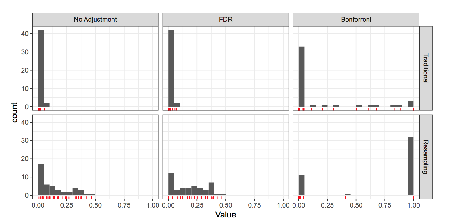
see the code: Bonferroni and FDR adj
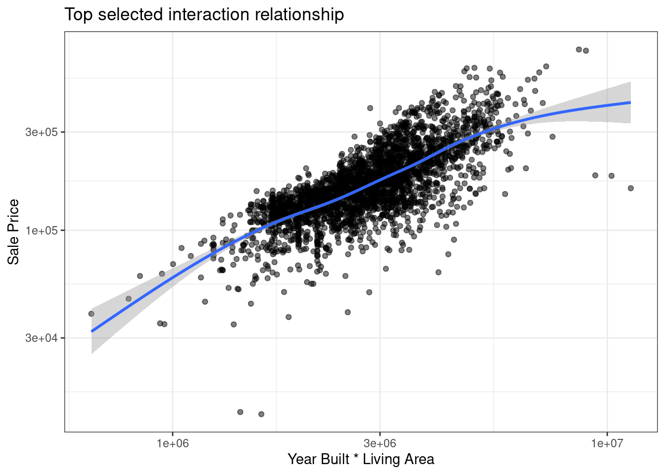
For example, in case of the Ames data, using resampling and choosing the potential interaction with the smallest p-value, latitude and longitude appear to be interesting interaction factors, but this would require more investigations, to understand if this interaction is significant.
The next step would be to compare the nested models with the ANOVA method.
see an example: “comparisons_nested_models.R”
7.5.2 Penalized Regression
One-at-a-time fashion evaluation of interaction terms, creates interaction terms to be added in the dataset. This method increases the number of predictors.
Models to use when there are more predictors than observations:
- trees
- svm
- neural networks
- k-nearest neighbors
- penalized models (less interpretable, but allow for linear/logistic regression)
How do we start with evaluating regression models?
Minimize sum of squared errors \[SSE=\sum_{i=1}^n{(y_i-\hat{y_i})^2}\]
\[\hat{y_i}=\hat{\beta_1}x_1+\hat{\beta_2}x_2+...+\hat{\beta_p}x_p\]
In case of penalized models:
Ridge regression: \(\lambda_r\) is called a penalty. To achieve better results, as regression coefficients grow large, the level of the penalty should rise. The penalty causes the resulting regression coefficients to become smaller and shrink towards zero. For combating collinearity. \[SSE=\sum{i=1}^n{(y_i-\hat{y_i})^2}+\lambda_r\sum_{j=1}^P{\beta_j^2}\]
Lasso: the least absolute shrinking, a modification to the ridge optimization criteria for the selection of predictors.
\[SSE=\sum{i=1}^n{(y_i-\hat{y_i})^2}+\lambda_l\sum_{j=1}^P{|\beta_j|}\]
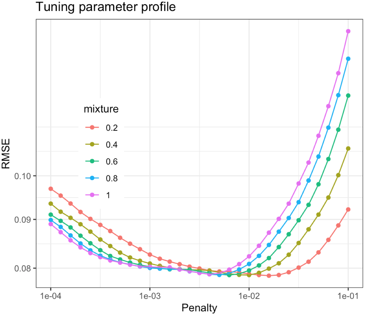
Approaches for blending both types of penalties together: glmnet model
\[\lambda=\lambda_r+\lambda_l\] where is \(\alpha\) is the proportion of \(\lambda\) associated with lasso penalty:
- full lasso: \(\alpha=1\)
- mix: \(\alpha=0.5\)
- full ridge: \(\alpha=0\)
\[SSE=\sum_{i=1}^n{(y_i-\hat{y_i})^2}+\lambda [(1-\alpha)\sum_{j=1}^P{\beta_j^2+\alpha\sum_{j=1}^P{|\beta_j|}]}\]