4.4 Preliminary exploratory visualizations

Ridership line plot by month

g1 <- train_plot_data %>% 
     select(date, rides = s_40380) %>% 
     mutate(date = floor_date(date, "month")) %>% 
     arrange(date) %>% 
     group_by(date) %>% 
     summarise(rides = sum(rides), .groups = 'drop') %>% 
     ggplot(aes(date, rides)) + 
     geom_line(size = 1) + 
     geom_smooth(method = 'loess', se = FALSE, color = 'steelblue') + 
     scale_x_date(date_labels = "%b-%Y", date_breaks  ="2 year")+
     labs(x = '', 
          y = "Rides (000's)", 
          title = 'Chicago Clark/Lake Train Station Monthly Ridership Volume (Jan 2001 - Aug 2016)'
     ) + 
     theme(axis.text.x = element_text(angle = 60, hjust = 1))

ggplotly(g1)

## `geom_smooth()` using formula = 'y ~ x'

Boxplot rides by day of the week

g2 <- train_plot_data %>% 
     select(dow, rides = s_40380) %>% 
     ggplot(aes(dow, rides, fill = dow)) + 
     geom_boxplot() + 
     labs(x = '', 
          y = "Rides (000's)", 
          title = 'Chicago Clark/Lake Train Station Ridership by Day of the Week') + 
     theme(legend.position = 'none')

ggplotly(g2)

Violinplot rides by day of the week

train_plot_data %>% 
     select(dow, rides = s_40380) %>% 
     ggplot(aes(dow, rides, fill = dow)) + 
     geom_violin() + 
     labs(x = '', 
          y = "Rides (000's)", 
          title = 'Chicago Clark/Lake Train Station Ridership by Day of the Week') + 
     theme(legend.position = 'none')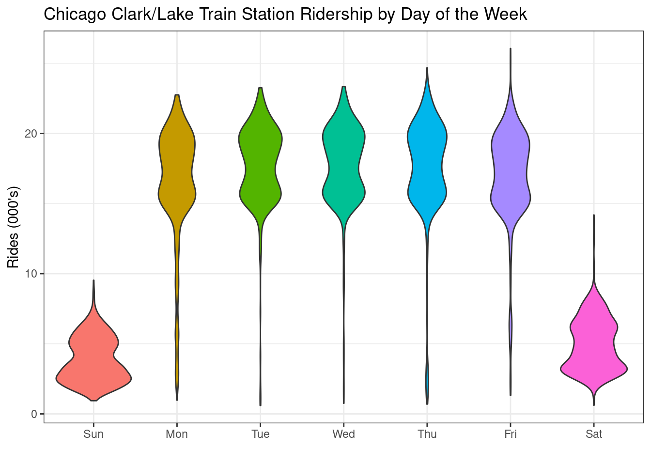

Boxplot rides by month

g3 <- train_plot_data %>% 
     select(month, rides = s_40380) %>% 
     ggplot(aes(month, rides, fill = month)) + 
     geom_boxplot() + 
     labs(x = '', 
          y = "Rides (000's)", 
          title = 'Chicago Clark/Lake Train Monthly Station Ridership') + 
     theme(legend.position = 'none')

ggplotly(g3)