6.1 Problematic Characteristics of predictors

One of the first things we can do when transforming our data is to rescale it to improve model performance. There are several different methods that can be used in different situations. Box-Cox and Yeo Johnson transformations can be used to correct for highly skewed predictors. Standardizing strategies such as scaling, centering, and smoothing can also be used to ensure your predictors have similar qualities.

6.1.1 Dealing with Skewed Data

Do a Box-Cox Transformation!

Originally developed to transform the outcome variable, box-cox uses maximum likelihood estimation to estimate a transformation parameter λ. The transformation allows the data to follow a normal distribution. The plot below shows the before and after effects.

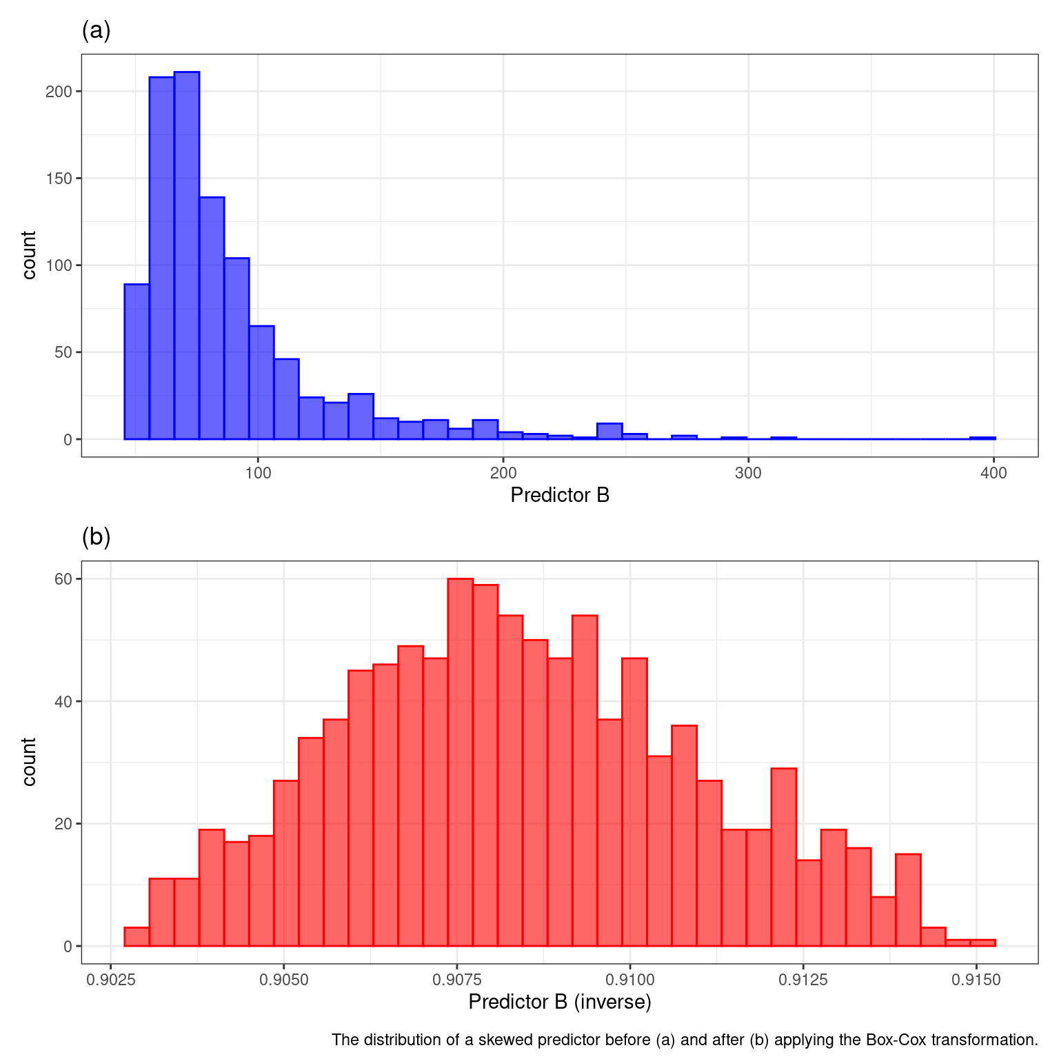
6.1.1.1 What does a Box-Cox transformation do?

Because the estimated parameter is in the exponent, it is called a POWER transformation. Different values of the parameter mimick no transformation (1), log transformation (0), square root (0.5), or inverse (-1). Because it is so flexible it can handle many different types of distributions

• Several caveats:

  • Can only be used when predictors are greater or equal to 0

  • Yeo-Johnson transformation can be used when there are negative values.

  • Best used for models that use polynomial transformations like linear regression, neural networks, or support vector machines.
    

6.1.1.2 Logit Transformation

Proportions, or data that falls between 0 and 1, are a special case that warrants their own transformation! Sometimes when a proportion is the outcome variable, model predictions can include results that are outside these bounds. Using a logit transformation, we can correct for that by changing the values between negative and positive infinity. If π is the variable, the logit transformations is:

\[ logit(π) = log(\frac{π}{1-π}) \]

After the predictions are calculated, you can use the inverse logit to return the data to its original form.

6.1.2 Standardizing

Why standardize? When your predictors are all in different units, with varying ranges, some may have an out-sized influence on the outcome when that should not be the case. This is especially true for models that use a distance computation like kNN, PCA, SVM, lasso and ridge regression, and variable importance calculation. Logistic regression and tree based methods not so much….

The main techniques illustrated in the book are centering, scaling, and smoothing sequential (time) data.

6.1.2.1 Centering and Scaling

Centering is pretty straight forward. For each variable, every value is subtracted by its average. After which, all variables will have a mean of zero.

Scaling is the process of dividing a variable by the corresponding training set’s standard deviation. This ensures that that variables have a standard deviation of one.

In addition to improving model performance, centering and scaling can also help better interpret our models for a couple reasons

1. It is easier to interpret the y-intercept when the predictors have been centered and scaled

2. Centering allows for an easier interpretation of coefficients with different magnitudes
   

6.1.2.2 Time data: Smoothing

When your model uses sequential, or time related, there can be a lot of noise in your model. By computing a running average,or a running median, we can smooth out our predictor and reduce noise. These are computed by taking the average of a point and one point before and after. The size of the moving window is extremely important. Small windows might not involve much smoothing at all, and large windows may miss out on important trends.

Computing the running median is especially important when there are major outliers in your sequential data.

A sequence of outcome values over time. The raw data contain outliers on days 10 and 45. The smoothed values are the result of a 3-point running median.