2.3 Example 2

Code for Section 2.4 at https://bookdown.org/max/FES/stroke-tour.html#stroke-exploration

Code to compare 2-way interaction models to their main effects model

a and b are two models from train()

compare_models_1way <- function(a, b, metric = a$metric[1], ...) {
  mods <- list(a, b)
  rs <- resamples(mods)
  diffs <- diff(rs, metric = metric[1], ...)
  diffs$statistics[[1]][[1]]
}

risk_preds is contained in the original data file and has the predictor names for the risk related variables

2.3.1 Create a “null model” with no predictors to get baseline performance

Compare the models with single predictors to the risk model. These data make

https://bookdown.org/max/FES/stroke-tour.html#tab:stroke-strokeRiskAssociations

VC_preds and risk_preds contain the predictor names for different sets.

one_predictor_res <- 
  data.frame(Predictor = c(VC_preds, risk_preds), 
             Improvement = NA,
             Pvalue = NA,
             ROC = NA,
             stringsAsFactors = FALSE)


for (i in 1:nrow(one_predictor_res)) {
  set.seed(63331)
  var_mod <- train(Stroke ~ ., 
                   data = stroke_train[, c("Stroke", one_predictor_res$Predictor[i])], 
                   method = "glm", 
                   metric = "ROC",
                   trControl = ctrl)  
  tmp_diff <- compare_models_1way(var_mod, 
                                  null_mod, 
                                  alternative = "greater")
  one_predictor_res$ROC[i] <- getTrainPerf(var_mod)[1, "TrainROC"]
  one_predictor_res$Improvement[i] <- tmp_diff$estimate
  one_predictor_res$Pvalue[i] <- tmp_diff$p.value
}

2.3.2 With Tidymodels

attempting this with tidymodels, not exactly the same need to make some sort of resample object to feed workflow_map

model_folds <- vfold_cv(tidy_training, v = 10, repeats = 5)
# model_boots <- bootstraps(tidy_training, times = 50) #want to bootstrap this?

#defining the null model
null_class_model <- 
    null_model() %>%
    set_engine("parsnip") %>%
    set_mode("classification")

null_model <- workflow_set(preproc = c(Stroke ~ .), 
                           models = list(null_mod = null_class_model))

# defining the model
lm_model <- 
  logistic_reg(
  mode = "classification", # outcome is a classification Stroke Y/N
  engine = "glm",   #using glm like the example
  penalty = NULL,   
  mixture = NULL        
)

# make named list of single variable formulae
single_var_formulae <-
    c(VC_preds, risk_preds) %>%
    paste0("Stroke ~ ", .) %>%
    set_names(., c(VC_preds, risk_preds)) %>%
    as.list() %>%
    map(., as.formula)

Create the workflow set, all of our models use the same type of model and input data

single_var_models <- workflow_set(preproc = single_var_formulae, 
                                     models = list(lm = lm_model))

all_models <- bind_rows(null_model, single_var_models)

# control grid/resamples allow processing of resampled data and parallel processing
# here we are asking only to save the predictions
control <- control_resamples(save_pred = TRUE)

doParallel::registerDoParallel()
all_models1 <- 
    all_models %>%
    #map over each model and its resamples, use the control parameters, and be noisy
    workflow_map(., 
                 resamples = model_folds, 
                 control = control, 
                 verbose = TRUE)

# save(all_models1, file = "data/all_models1.RData", compress = "xz")

# per model what are the predictions, summmarize over resamples
collect_predictions(all_models1, summarize = TRUE)

## # A tibble: 2,492 × 9
##    wflow_id         .config   preproc model  .row Stroke .pred_N .pred_Y .pred…¹
##    <chr>            <fct>     <chr>   <chr> <int> <fct>    <dbl>   <dbl> <fct>  
##  1 formula_null_mod Preproce… formula null…     1 N        0.495   0.505 Y      
##  2 formula_null_mod Preproce… formula null…     2 N        0.478   0.522 Y      
##  3 formula_null_mod Preproce… formula null…     3 N        0.495   0.505 Y      
##  4 formula_null_mod Preproce… formula null…     4 N        0.475   0.525 Y      
##  5 formula_null_mod Preproce… formula null…     5 N        0.485   0.515 Y      
##  6 formula_null_mod Preproce… formula null…     6 N        0.498   0.502 Y      
##  7 formula_null_mod Preproce… formula null…     7 N        0.488   0.512 Y      
##  8 formula_null_mod Preproce… formula null…     8 N        0.485   0.515 Y      
##  9 formula_null_mod Preproce… formula null…     9 N        0.491   0.509 Y      
## 10 formula_null_mod Preproce… formula null…    10 N        0.482   0.518 Y      
## # … with 2,482 more rows, and abbreviated variable name ¹​.pred_class

# per model what are the outputs in terms of fit (auc_roc) and accuracy 
collect_metrics(all_models1)

## # A tibble: 56 × 9
##    wflow_id         .config    preproc model .metric .esti…¹  mean     n std_err
##    <chr>            <fct>      <chr>   <chr> <chr>   <chr>   <dbl> <int>   <dbl>
##  1 formula_null_mod Preproces… formula null… accura… binary  0.378    50  0.0131
##  2 formula_null_mod Preproces… formula null… roc_auc binary  0.5      50  0     
##  3 CALCVol_lm       Preproces… formula logi… accura… binary  0.388    50  0.0183
##  4 CALCVol_lm       Preproces… formula logi… roc_auc binary  0.457    50  0.0291
##  5 CALCVolProp_lm   Preproces… formula logi… accura… binary  0.441    50  0.0196
##  6 CALCVolProp_lm   Preproces… formula logi… roc_auc binary  0.502    50  0.0260
##  7 MATXVol_lm       Preproces… formula logi… accura… binary  0.346    50  0.0177
##  8 MATXVol_lm       Preproces… formula logi… roc_auc binary  0.380    50  0.0277
##  9 MATXVolProp_lm   Preproces… formula logi… accura… binary  0.415    50  0.0222
## 10 MATXVolProp_lm   Preproces… formula logi… roc_auc binary  0.516    50  0.0285
## # … with 46 more rows, and abbreviated variable name ¹​.estimator

# plot the output to show which individual parameters have the most impact
autoplot(
   all_models1,
   rank_metric = "roc_auc",  # <- how to order models
   metric = "roc_auc",       # <- which metric to visualize
   select_best = FALSE     # <- one point per workflow
) +
   geom_text(aes(y = mean - 1/10*mean, 
                 label = wflow_id),
             angle = 90, hjust = 1) +
   theme(legend.position = "none")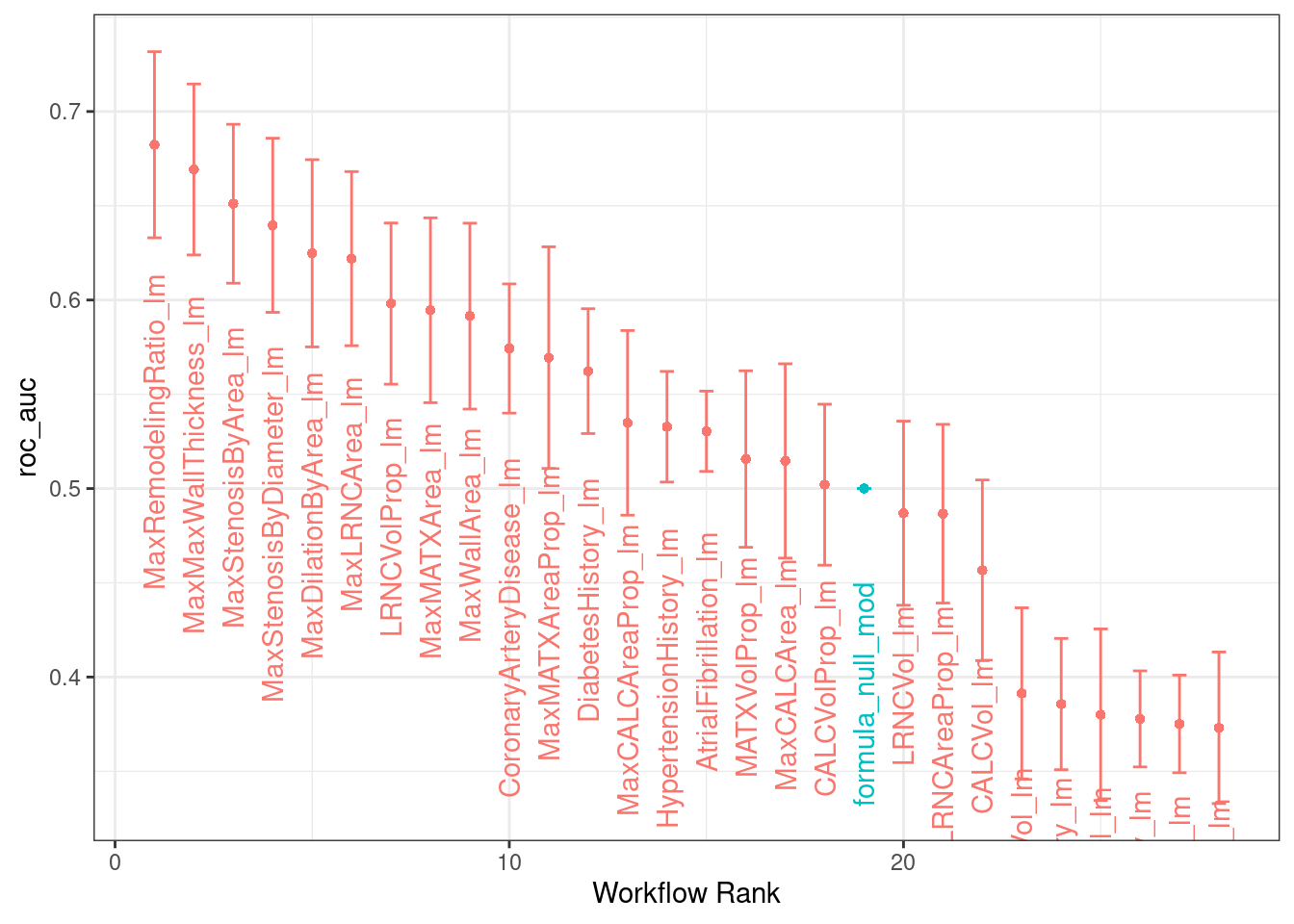

# per model, sort by auc_roc
all_models1 %>%
rank_results() %>% 
   filter(.metric == "roc_auc")

## # A tibble: 28 × 9
##    wflow_id              .config .metric  mean std_err     n prepr…¹ model  rank
##    <chr>                 <fct>   <chr>   <dbl>   <dbl> <int> <chr>   <chr> <int>
##  1 MaxRemodelingRatio_lm Prepro… roc_auc 0.682  0.0300    50 formula logi…     1
##  2 MaxMaxWallThickness_… Prepro… roc_auc 0.669  0.0276    50 formula logi…     2
##  3 MaxStenosisByArea_lm  Prepro… roc_auc 0.651  0.0256    50 formula logi…     3
##  4 MaxStenosisByDiamete… Prepro… roc_auc 0.640  0.0281    50 formula logi…     4
##  5 MaxDilationByArea_lm  Prepro… roc_auc 0.625  0.0302    50 formula logi…     5
##  6 MaxLRNCArea_lm        Prepro… roc_auc 0.622  0.0281    50 formula logi…     6
##  7 LRNCVolProp_lm        Prepro… roc_auc 0.598  0.0260    50 formula logi…     7
##  8 MaxMATXArea_lm        Prepro… roc_auc 0.595  0.0298    50 formula logi…     8
##  9 MaxWallArea_lm        Prepro… roc_auc 0.591  0.0300    50 formula logi…     9
## 10 CoronaryArteryDiseas… Prepro… roc_auc 0.574  0.0208    50 formula logi…    10
## # … with 18 more rows, and abbreviated variable name ¹​preprocessor

# Data in table 2.3
# https://bookdown.org/max/FES/stroke-tour.html#tab:stroke-strokeRiskAssociations

one_predictor_res %>% 
  dplyr::filter(Predictor %in% risk_preds) %>% 
  arrange(Pvalue)

##                     Predictor Improvement       Pvalue      ROC
## 1       CoronaryArteryDisease    0.079000 0.0002957741 0.579000
## 2             DiabetesHistory    0.066500 0.0003019908 0.566500
## 3         HypertensionHistory    0.065000 0.0004269919 0.565000
## 4                         age    0.082975 0.0011215271 0.582975
## 5          AtrialFibrillation    0.044000 0.0013131334 0.544000
## 6              SmokingHistory   -0.015000 0.7372947489 0.485000
## 7                         sex   -0.029000 0.8970159364 0.471000
## 8 HypercholesterolemiaHistory   -0.101000 0.9999998987 0.399000

# Figure 2.4
# https://bookdown.org/max/FES/stroke-tour.html#fig:stroke-vascuCAPAssocations

vc_pred <- 
  recipe(Stroke ~ ., data = stroke_train %>% dplyr::select(Stroke, !!!VC_preds)) %>% 
    step_YeoJohnson(all_predictors()) %>% 
    prep(stroke_train %>% dplyr::select(Stroke, !!!VC_preds)) %>% 
    bake(., new_data = NULL) %>% 
    gather(Predictor, value, -Stroke)
vc_pred%>%head

## # A tibble: 6 × 3
##   Stroke Predictor value
##   <fct>  <chr>     <dbl>
## 1 N      CALCVol    9.51
## 2 N      CALCVol    4.90
## 3 N      CALCVol    7.63
## 4 Y      CALCVol   13.2 
## 5 N      CALCVol    6.93
## 6 N      CALCVol    2.27

pred_max <- 
  vc_pred %>% 
  group_by(Predictor) %>% 
  summarize(max_val = max(value)) %>% 
  inner_join(one_predictor_res %>% dplyr::select(Pvalue, Predictor)) %>% 
  mutate(
    x = 1.5, 
    value = 1.25 * max_val,
    label = paste0("p-value: ", format.pval(Pvalue, digits = 2, sci = FALSE, eps = .0001))
  )

## Joining, by = "Predictor"

pred_max%>%head

## # A tibble: 6 × 6
##   Predictor     max_val   Pvalue     x     value label           
##   <chr>           <dbl>    <dbl> <dbl>     <dbl> <chr>           
## 1 CALCVol        15.7   0.000872   1.5    19.6   p-value: 0.00087
## 2 CALCVolProp     0.440 0.000856   1.5     0.550 p-value: 0.00086
## 3 LRNCVol        23.2   1.00       1.5    29.0   p-value: 1.00000
## 4 LRNCVolProp     0.495 0.207      1.5     0.618 p-value: 0.20723
## 5 MATXVol     41681.    1.00       1.5 52101.    p-value: 1.00000
## 6 MATXVolProp     0.870 1.00       1.5     1.09  p-value: 1.00000

new_order <- pred_max$Predictor[order(pred_max$Pvalue)]

vc_pred <- 
  vc_pred %>% 
  mutate(Predictor = factor(Predictor, levels = new_order))

pred_max <- 
  pred_max %>% 
  mutate(Predictor = factor(Predictor, levels = new_order))

fig_2_4 <-
  ggplot(vc_pred, aes(x = Stroke, y = value)) + 
  geom_boxplot() + 
  geom_point(alpha = 0.3, cex = .5) + 
  geom_text(data = pred_max, aes(x = x, label = label), size = 3) + 
  facet_wrap(~Predictor, scales = "free_y") + 
  ylab("")
fig_2_4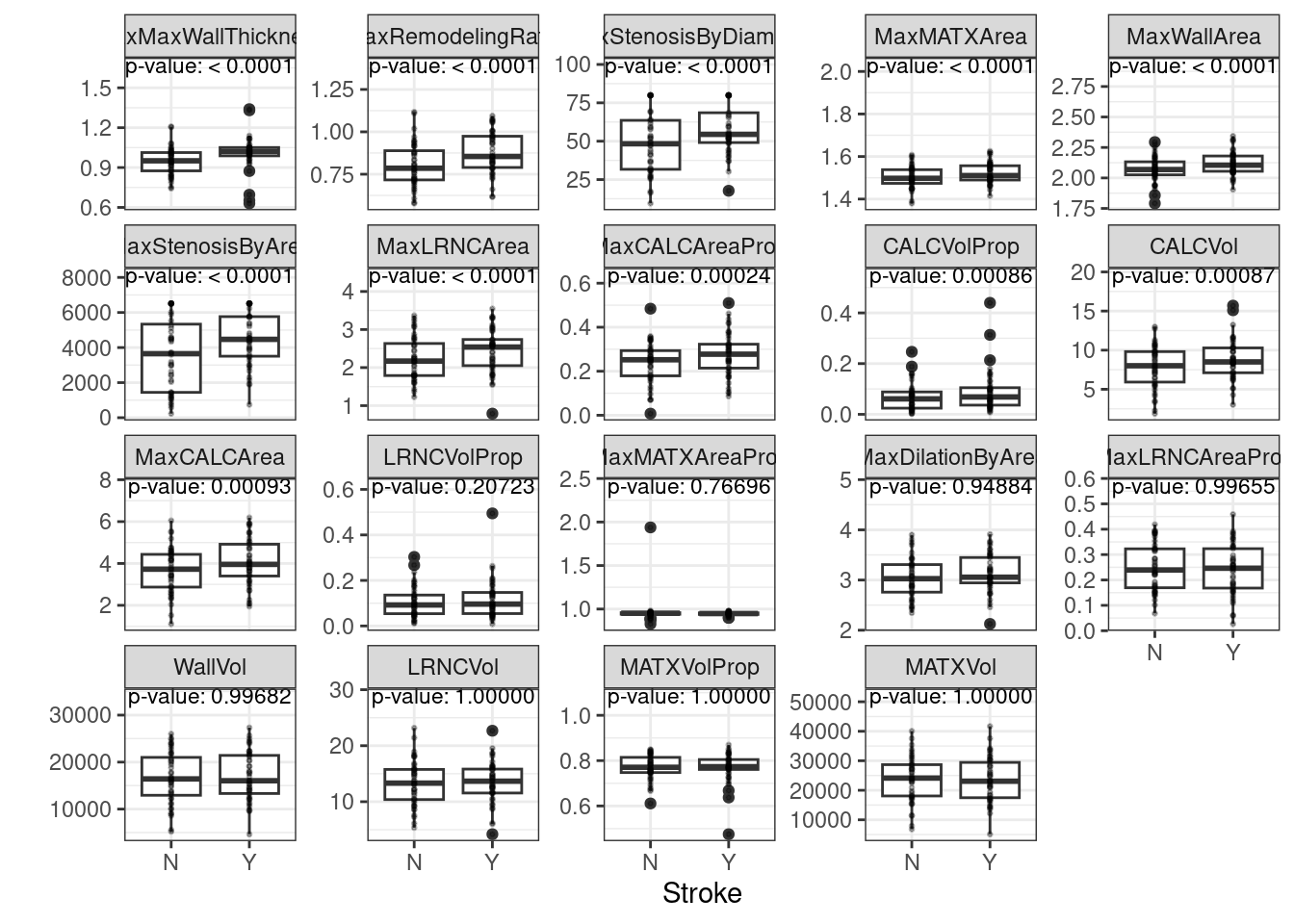

# Figure 2.5
# https://bookdown.org/max/FES/stroke-tour.html#fig:stroke-maxRemodelingRatioROC

fig_2_5 <- 
  roc_curve(stroke_train, Stroke, MaxRemodelingRatio) %>% 
  # used opposite values
  ggplot(aes(x = specificity, y = 1-sensitivity)) + 
  geom_abline(alpha = .5, lty = 2) +
  geom_path()

fig_2_5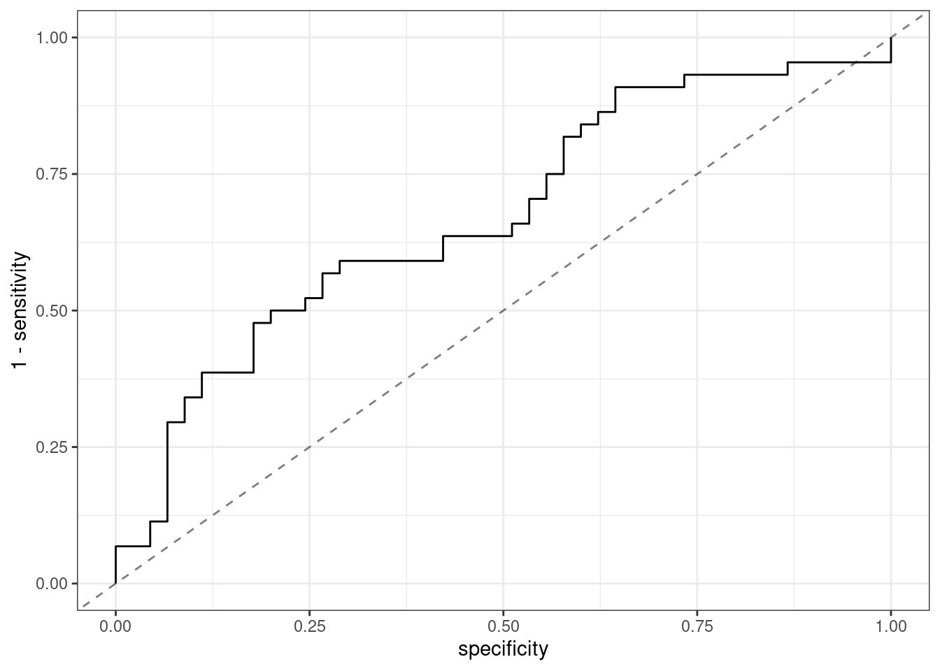

2.3.3 Interaction exploration

Here they create all the pairs of all of the image analysis components there are 171 interactions

pairs <- 
  combn(VC_preds, 2) %>% 
  t() %>% 
  as.data.frame(stringsAsFactors = FALSE) %>% 
  mutate(
    Improvement = NA,
    Pvalue = NA,
    ROC = NA
  )

Run comparisons with caret

retained_pairs <- 
  pairs1 %>% 
  dplyr::filter(ROC > 0.5  & Pvalue <= 0.2)
retained_pairs%>%head

##        V1                    V2 Improvement      Pvalue     ROC
## 1 MATXVol   MaxMaxWallThickness     0.07635 0.001903838 0.65435
## 2 MATXVol    MaxRemodelingRatio     0.11085 0.001345363 0.55150
## 3 MATXVol     MaxStenosisByArea     0.02325 0.086210254 0.60960
## 4 MATXVol MaxStenosisByDiameter     0.01930 0.197228736 0.61550
## 5 LRNCVol           MaxMATXArea     0.02590 0.152003535 0.55690
## 6 LRNCVol    MaxRemodelingRatio     0.03345 0.119774508 0.59510

# Figure 2.6
# https://bookdown.org/max/FES/stroke-tour.html#fig:stroke-interactionScreening

vol_plot <- 
  pairs1 %>% 
  dplyr::filter(ROC > 0.5) %>%
  mutate(Term = paste(V1, "by", V2, "\nROC:", round(ROC, 2))) %>%
  ggplot(aes(x = Improvement, y = -log10(Pvalue))) + 
  xlab("Improvement") +
  geom_point(alpha = .2, aes(size = ROC, text = Term))

vol_plot <- ggplotly(vol_plot, tooltip = "Term")
vol_plot

Create interaction formula of things that matter most

int_form <- 
  pairs1 %>% 
  dplyr::filter(ROC > 0.5  & Pvalue <= 0.2 & Improvement > 0) %>% 
  mutate(form  = paste0(V1, ":", V2)) %>% 
  pull(form) %>% 
  paste(collapse = "+")

int_form <- paste("~", int_form)
int_form <- as.formula(int_form)
int_form%>%head

## ~MATXVol:MaxMaxWallThickness + MATXVol:MaxRemodelingRatio + MATXVol:MaxStenosisByArea + 
##     MATXVol:MaxStenosisByDiameter + LRNCVol:MaxMATXArea + LRNCVol:MaxRemodelingRatio + 
##     MaxCALCAreaProp:MaxMATXAreaProp + MaxCALCAreaProp:MaxRemodelingRatio + 
##     MaxDilationByArea:MaxMaxWallThickness + MaxDilationByArea:MaxRemodelingRatio + 
##     MaxMATXAreaProp:MaxLRNCArea + MaxMATXAreaProp:MaxRemodelingRatio + 
##     MaxMATXAreaProp:MaxWallArea + MaxMaxWallThickness:MaxStenosisByArea + 
##     MaxMaxWallThickness:WallVol + MaxRemodelingRatio:MaxWallArea + 
##     MaxRemodelingRatio:WallVol + MaxStenosisByArea:WallVol

This part of the script is to work through all of of the potential models:

• original risk set alone
• imaging predictors alone
• risk and imaging predictors together
• imaging predictors and interactions of imaging predictors, and
• risk, imaging predictors, and interactions of imaging predictors

All the models are run below.

risk_train <- 
  stroke_train %>%
  dplyr::select(one_of(risk_preds), Stroke)

risk_train%>%head

##   age sex SmokingHistory AtrialFibrillation CoronaryArteryDisease
## 1  72   1              1                  0                     0
## 2  76   1              1                  0                     0
## 4  72   0              0                  0                     0
## 5  61   1              1                  0                     0
## 7  65   1              0                  0                     0
## 8  64   1              1                  0                     1
##   DiabetesHistory HypercholesterolemiaHistory HypertensionHistory Stroke
## 1               0                           0                   1      N
## 2               1                           1                   1      N
## 4               0                           0                   0      N
## 5               1                           1                   1      Y
## 7               0                           0                   1      N
## 8               0                           1                   1      N

image_train <- 
  stroke_train %>%
  dplyr::select(one_of(VC_preds), Stroke)

image_train%>%head

##      CALCVol CALCVolProp  MATXVol MATXVolProp   LRNCVol LRNCVolProp MaxCALCArea
## 1 235.252599 0.070442702 3156.835   0.7599582 224.87171  0.09108513   12.350494
## 2  31.433595 0.016164769 3032.861   0.8133063 368.56066  0.13398944    7.130660
## 4 113.404823 0.038081488 3835.220   0.7825256 321.15893  0.08303659   16.286916
## 5 780.823789 0.213432061 3518.877   0.7610895 140.51735  0.03206536   63.350869
## 7  84.055774 0.041383842 2990.273   0.7498691 293.26992  0.07539753   17.583561
## 8   5.644322 0.002824946 3359.323   0.8492801  55.76888  0.01983567    2.841252
##   MaxCALCAreaProp MaxDilationByArea MaxMATXArea MaxMATXAreaProp MaxLRNCArea
## 1      0.36576842         520.98259    71.24743       0.9523705   21.686815
## 2      0.21124686          91.72005    27.21084       0.9455539    6.434661
## 4      0.40881121         270.96930    38.12211       0.9459098    5.705054
## 5      0.57620574        2270.45120   341.12089       0.9691989    6.046787
## 7      0.32150685          95.15505    56.57457       0.9213197    7.213451
## 8      0.07734609         298.42121    33.92709       0.9612049    4.595196
##   MaxLRNCAreaProp MaxMaxWallThickness MaxRemodelingRatio MaxStenosisByArea
## 1       0.4295781            2.409943           5.697931          18.99554
## 2       0.2815101            2.540334           1.739927          30.23761
## 4       0.1547786            3.708515           2.831636          33.93906
## 5       0.1870965            6.115838          15.647750          34.30985
## 7       0.2169263            3.975168           1.912069          36.59954
## 8       0.2053274            2.581908           2.181675          40.31766
##   MaxWallArea  WallVol MaxStenosisByDiameter Stroke
## 1   106.20676 4192.170              10.54411      N
## 2    33.36714 3917.040              18.64620      N
## 4    55.34671 4935.327              19.73511      N
## 5   426.47858 4909.504              20.28832      Y
## 7    59.82696 4045.053              49.29705      N
## 8    34.79742 3960.832              30.50857      N

fiveStats <- function(...) c(twoClassSummary(...), defaultSummary(...))
internal_ctrl = trainControl(method = "none", classProbs = TRUE,
                             allowParallel = FALSE)
lrFuncsNew <- caretFuncs  
lrFuncsNew$summary <- fiveStats
rfeCtrl <- rfeControl(functions = lrFuncsNew,
                      method = "repeatedcv",
                      repeats = 5,
                      rerank = FALSE,
                      returnResamp = "all",
                      saveDetails = TRUE,
                      verbose = FALSE)

RFE procedure using risk predictors

All pair-wise interactions.

risk_int_filtered_recipe <-
  recipe(Stroke ~ ., data = risk_train) %>%
  step_interact(~ all_predictors():all_predictors()) %>%
  step_corr(all_predictors(), threshold = 0.75) %>% 
  step_center(all_predictors()) %>%
  step_scale(all_predictors()) %>%
  step_zv(all_predictors())

set.seed(63331)
risk_int_filtered_rfe <- rfe(
  risk_int_filtered_recipe,
  data = risk_train,
  sizes = 1:36,
  rfeControl = rfeCtrl,
  metric = "ROC",
  ## train options
  method = "glm",
  trControl = internal_ctrl
)

# Main effects
risk_main_filtered_recipe <-
  recipe(Stroke ~ ., data = risk_train) %>%
  step_corr(all_predictors(), threshold = 0.75) %>% 
  step_center(all_predictors()) %>%
  step_scale(all_predictors()) %>%
  step_zv(all_predictors())

set.seed(63331)
risk_main_filtered_rfe <- rfe(
  risk_main_filtered_recipe,
  data = risk_train,
  sizes = 1:8,
  rfeControl = rfeCtrl,
  metric = "ROC",
  ## train options
  method = "glm",
  trControl = internal_ctrl
)

RFE procedure using imaging predictors.

img_int_filtered_recipe <-
  recipe(Stroke ~ ., data = image_train) %>%
  step_interact(int_form)  %>%
  step_corr(all_predictors(), threshold = 0.75) %>%
  step_center(all_predictors()) %>%
  step_scale(all_predictors()) %>%
  step_YeoJohnson(all_predictors()) %>%
  step_zv(all_predictors())

set.seed(63331)
img_int_filtered_rfe <- rfe(
  img_int_filtered_recipe,
  data = image_train,
  sizes = 1:35,
  rfeControl = rfeCtrl,
  metric = "ROC",
  ## train options
  method = "glm",
  trControl = internal_ctrl
)

img_main_filtered_recipe <-
  recipe(Stroke ~ ., data = image_train)  %>%
  step_corr(all_predictors(), threshold = 0.75) %>%
  step_center(all_predictors()) %>%
  step_scale(all_predictors()) %>%
  step_YeoJohnson(all_predictors()) %>%
  step_zv(all_predictors())

set.seed(63331)
img_main_filtered_rfe <- rfe(
  img_main_filtered_recipe,
  data = image_train,
  sizes = 1:19,
  rfeControl = rfeCtrl,
  metric = "ROC",
  ## train options
  method = "glm",
  trControl = internal_ctrl
)

both_int_filtered_recipe <-
  recipe(Stroke ~ ., data = stroke_train) %>%
  step_interact(int_form)  %>%
  step_corr(all_predictors(), threshold = 0.75) %>%
  step_center(all_predictors()) %>%
  step_scale(all_predictors()) %>%
  step_YeoJohnson(all_predictors()) %>%
  step_zv(all_predictors())

set.seed(63331)
both_int_filtered_rfe <- rfe(
  both_int_filtered_recipe,
  data = stroke_train,
  sizes = 1:44,
  rfeControl = rfeCtrl,
  metric = "ROC",
  ## train options
  method = "glm",
  trControl = internal_ctrl
)

both_main_filtered_recipe <-
  recipe(Stroke ~ ., data = stroke_train)  %>%
  step_corr(all_predictors(), threshold = 0.75) %>%
  step_center(all_predictors()) %>%
  step_scale(all_predictors()) %>%
  step_YeoJohnson(all_predictors()) %>%
  step_zv(all_predictors())

set.seed(63331)
both_main_filtered_rfe <- rfe(
  both_main_filtered_recipe,
  data = stroke_train,
  sizes = 1:28,
  rfeControl = rfeCtrl,
  metric = "ROC",
  ## train options
  method = "glm",
  trControl = internal_ctrl
)

risk_int_recipe <-
  recipe(Stroke ~ ., data = risk_train) %>%
  step_interact(~ all_predictors():all_predictors()) %>%
  step_center(all_predictors()) %>%
  step_scale(all_predictors()) %>%
  step_zv(all_predictors())

set.seed(63331)
risk_int_rfe <- rfe(
  risk_int_recipe,
  data = risk_train,
  sizes = 1:36,
  rfeControl = rfeCtrl,
  metric = "ROC",
  ## train options
  method = "glm",
  trControl = internal_ctrl
)

risk_main_recipe <-
  recipe(Stroke ~ ., data = risk_train) %>%
  step_center(all_predictors()) %>%
  step_scale(all_predictors()) %>%
  step_zv(all_predictors())

set.seed(63331)
risk_main_rfe <- rfe(
  risk_main_recipe,
  data = risk_train,
  sizes = 1:8,
  rfeControl = rfeCtrl,
  metric = "ROC",
  ## train options
  method = "glm",
  trControl = internal_ctrl
)

img_int_recipe <-
  recipe(Stroke ~ ., data = image_train) %>%
  step_interact(int_form)  %>%
  step_center(all_predictors()) %>%
  step_scale(all_predictors()) %>%
  step_YeoJohnson(all_predictors()) %>%
  step_zv(all_predictors())

set.seed(63331)
img_int_rfe <- rfe(
  img_int_recipe,
  data = image_train,
  sizes = 1:35,
  rfeControl = rfeCtrl,
  metric = "ROC",
  ## train options
  method = "glm",
  trControl = internal_ctrl
)

img_main_recipe <-
  recipe(Stroke ~ ., data = image_train)  %>%
  step_center(all_predictors()) %>%
  step_scale(all_predictors()) %>%
  step_YeoJohnson(all_predictors()) %>%
  step_zv(all_predictors())

set.seed(63331)
img_main_rfe <- rfe(
  img_main_recipe,
  data = image_train,
  sizes = 1:19,
  rfeControl = rfeCtrl,
  metric = "ROC",
  ## train options
  method = "glm",
  trControl = internal_ctrl
)

both_int_recipe <-
  recipe(Stroke ~ ., data = stroke_train) %>%
  step_interact(int_form)  %>%
  step_center(all_predictors()) %>%
  step_scale(all_predictors()) %>%
  step_YeoJohnson(all_predictors()) %>%
  step_zv(all_predictors())

set.seed(63331)
both_int_rfe <- rfe(
  both_int_recipe,
  data = stroke_train,
  sizes = 1:44,
  rfeControl = rfeCtrl,
  metric = "ROC",
  ## train options
  method = "glm",
  trControl = internal_ctrl
)

both_main_recipe <-
  recipe(Stroke ~ ., data = stroke_train)  %>%
  step_center(all_predictors()) %>%
  step_scale(all_predictors()) %>%
  step_YeoJohnson(all_predictors()) %>%
  step_zv(all_predictors())

set.seed(63331)
both_main_rfe <- rfe(
  both_main_recipe,
  data = stroke_train,
  sizes = 1:28,
  rfeControl = rfeCtrl,
  metric = "ROC",
  ## train options
  method = "glm",
  trControl = internal_ctrl
)

format_data <- function(x, lab, int = FALSE) {
  dat <- 
    x %>% 
    pluck("results") %>% 
    mutate(Predictors = !!lab) %>% 
    dplyr::select(ROC, Variables, Predictors, Variables, Num_Resamples) %>% 
    mutate(Model = "Main Effects")
  if (int)
    dat$Model <- "Interactions"
  dat
  
}

filtered_dat <- 
  bind_rows(
    format_data(risk_main_filtered_rfe, lab = "Risk Predictors"),
    format_data(risk_int_filtered_rfe, lab = "Risk Predictors", TRUE),
    format_data(img_main_filtered_rfe, lab = "Imaging Predictors"),
    format_data(img_int_filtered_rfe, lab = "Imaging Predictors", TRUE),
    format_data(both_main_filtered_rfe, lab = "All Predictors"),
    format_data(both_int_filtered_rfe, lab = "All Predictors", TRUE)
  ) %>% 
  mutate(
    Predictors = factor(
      Predictors, 
      levels = c("Risk Predictors", "Imaging Predictors", "All Predictors")
    ),
    Model = factor(Model, levels = c("Main Effects", "Interactions")),
    Filtering = "Correlation Filter"
  )

unfiltered_dat <- 
  bind_rows(
    format_data(risk_main_rfe, lab = "Risk Predictors"),
    format_data(risk_int_rfe, lab = "Risk Predictors", TRUE),
    format_data(img_main_rfe, lab = "Imaging Predictors"),
    format_data(img_int_rfe, lab = "Imaging Predictors", TRUE),
    format_data(both_main_rfe, lab = "All Predictors"),
    format_data(both_int_rfe, lab = "All Predictors", TRUE)
  ) %>% 
  mutate(
    Predictors = factor(
      Predictors, 
      levels = c("Risk Predictors", "Imaging Predictors", "All Predictors")
    ),
    Model = factor(Model, levels = c("Main Effects", "Interactions")),
    Filtering = "No Filter"
  )

rfe_data <- 
  bind_rows(filtered_dat, unfiltered_dat) %>% 
  mutate(
    Filtering = factor(Filtering, levels = c("No Filter", "Correlation Filter"))
  )

# https://bookdown.org/max/FES/predictive-modeling-across-sets.html#fig:stroke-rfe-res
ggplot(rfe_data, aes(x = Variables, y = ROC, col = Model)) +
  geom_point(size = 0.75) + 
  geom_line() + 
  facet_grid(Filtering ~ Predictors) + 
  scale_color_manual(values = c("#6A3D9A", "#CAB2D6"))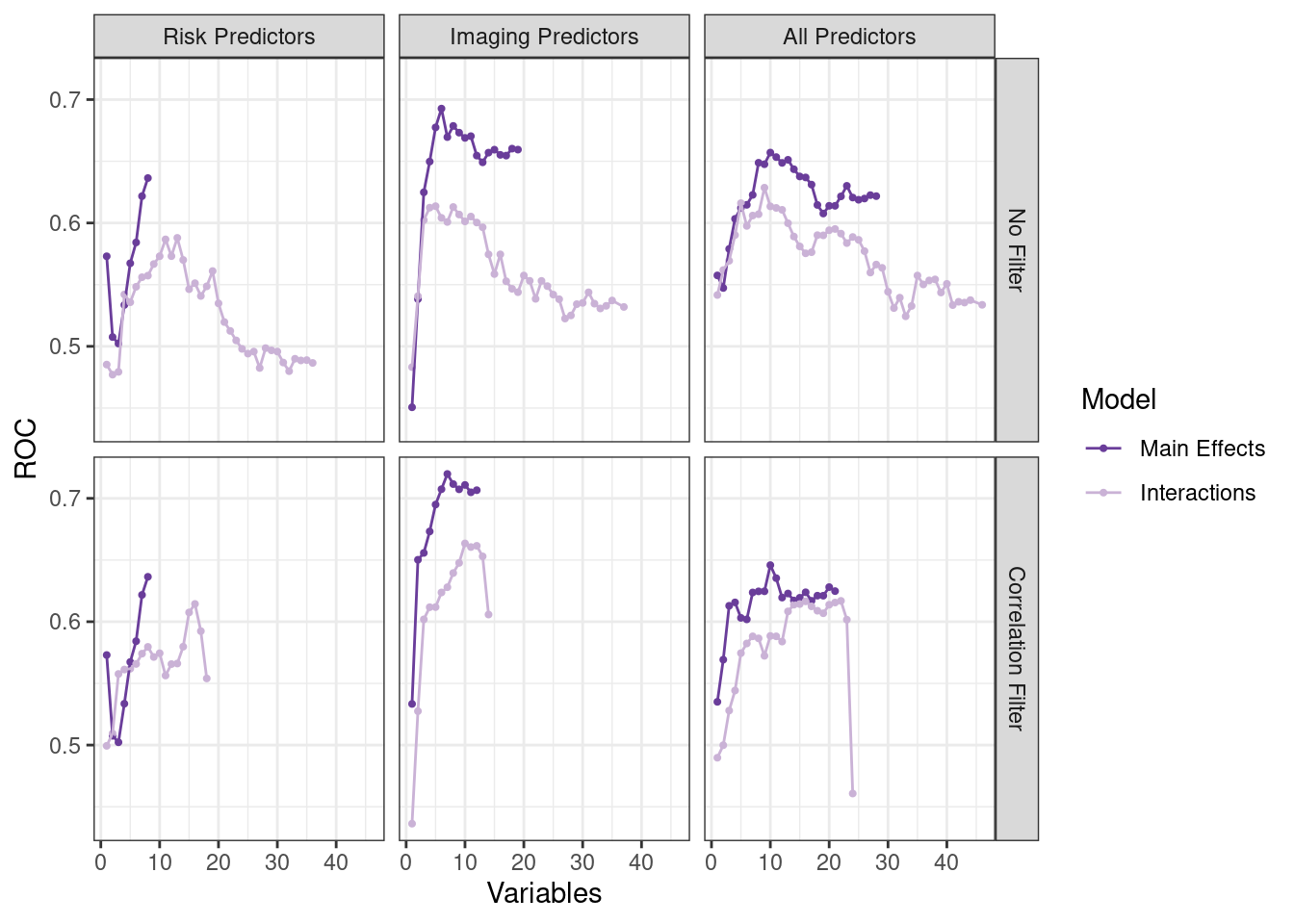

# https://bookdown.org/max/FES/predictive-modeling-across-sets.html#tab:stroke-rfe-tab
rfe_tab <-
  img_main_filtered_rfe %>% 
  pluck("variables") %>% 
  filter(Variables == img_main_filtered_rfe$optsize) %>% 
  group_by(var) %>% 
  count() %>% 
  arrange(desc(n)) %>% 
  mutate(final = ifelse(var %in% img_main_filtered_rfe$optVariables, "Yes", "No")) %>% 
  ungroup()