12.2 12.2 Simulated Annealing
Annealing is the process of heating a metal or glass to remove imperfections and improve strength in the material. The annealing process that happens to particles within a material can be abstracted and applied for the purpose of feature selection.
In the context of feature selection, features are particles. Simulated annealing works by iteritively testing how strong (predictive) each of the features are. After each iteration, the energy of the material (the features in your model) is testing tested for predictive power.
Additionally, during each iteration a new subset of features are included and compared to previous iterations. If the subset of features reaches a certain threshold of predictive power it is kept for the next iteration, if it doesn’t meet the threshold it is discarded.
The acceptance probability formula is as follows:
\(Pr[accept] = \exp\left[-\frac{i}{c}\left(\frac{old-new}{old}\right)\right]\)
To understand the acceptance probability formula, consider an example where the objective is to optimize predictive accuracy. Suppose the previous solution had an accuracy of 85% and the current solution had an accuracy of 80%. The proportionate decrease of the current solution relative to the previous solution is 0.059. If this situation occurred in the first iteration, then the acceptance probability would be 0.94. If this situation occurred at iteration 5, the probability of accepting the inferior subset would be 0.75%. At iteration 50, this the acceptance probability drops to 0.05. Therefore, the probability of accepting a worse solution decreases as the algorithm iteration increases.
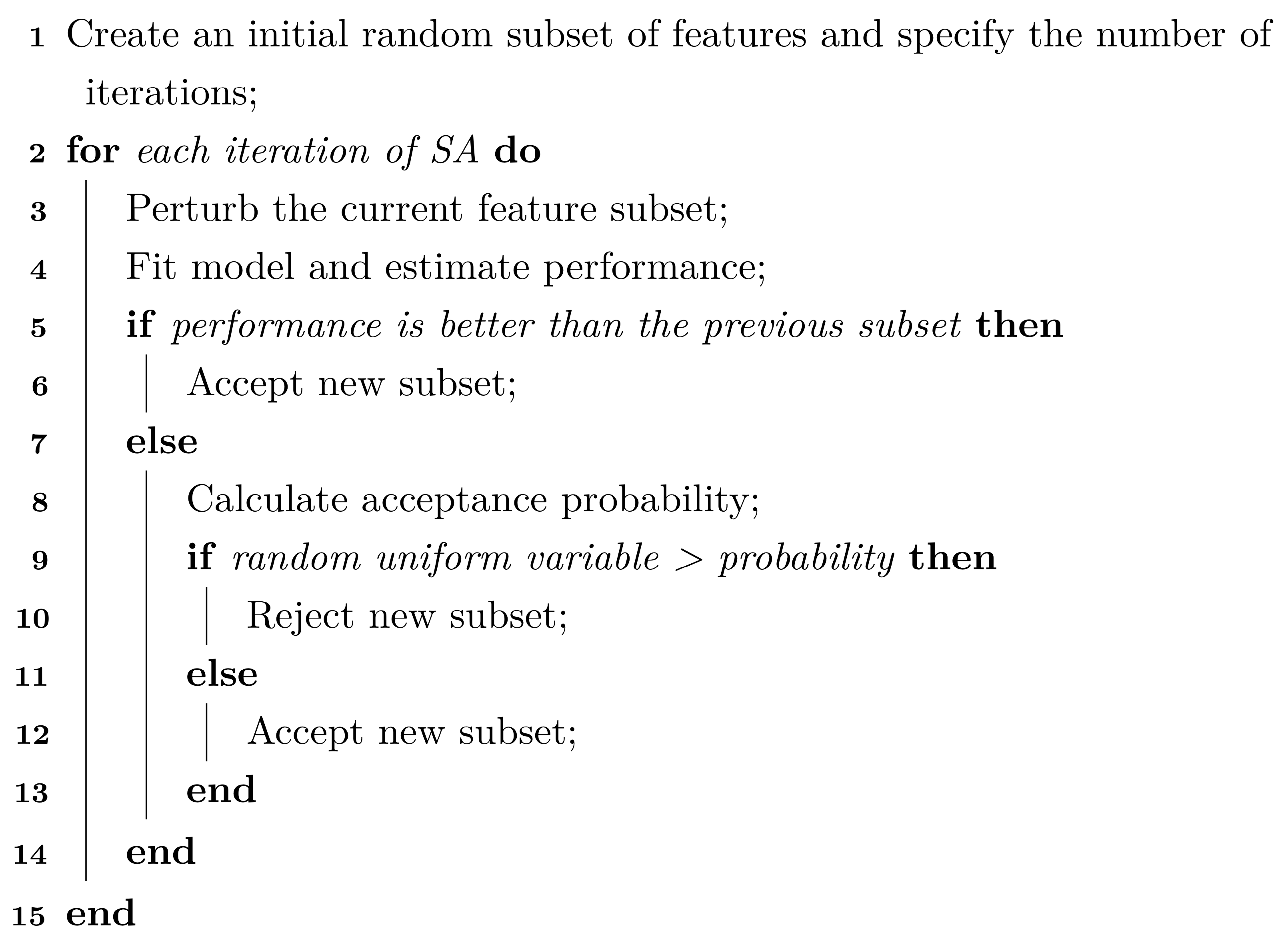
This algorithm summarizes the basic simulated annealing algorithm for feature selection:
The following is an example of how simulated annealing works across a number of iterations with a restart at iteration 14.
| Iteration | Size | ROC | Probability | Random Uniform | Status |
|---|---|---|---|---|---|
| 1 | 122 | 0.776 | — | — | Improved |
| 2 | 120 | 0.781 | — | — | Improved |
| 3 | 122 | 0.770 | 0.958 | 0.767 | Accepted |
| 4 | 120 | 0.804 | — | — | Improved |
| 5 | 120 | 0.793 | 0.931 | 0.291 | Accepted |
| 6 | 118 | 0.779 | 0.826 | 0.879 | Discarded |
| 7 | 122 | 0.779 | 0.799 | 0.659 | Accepted |
| 8 | 124 | 0.776 | 0.756 | 0.475 | Accepted |
| 9 | 124 | 0.798 | 0.929 | 0.879 | Accepted |
| 10 | 124 | 0.774 | 0.685 | 0.846 | Discarded |
| 11 | 126 | 0.788 | 0.800 | 0.512 | Accepted |
| 12 | 124 | 0.783 | 0.732 | 0.191 | Accepted |
| 13 | 124 | 0.790 | 0.787 | 0.060 | Accepted |
| 14 | 124 | 0.778 | — | — | Restart |
| 15 | 120 | 0.790 | 0.982 | 0.049 | Accepted |
12.2.1 Selecting Features without Overfitting
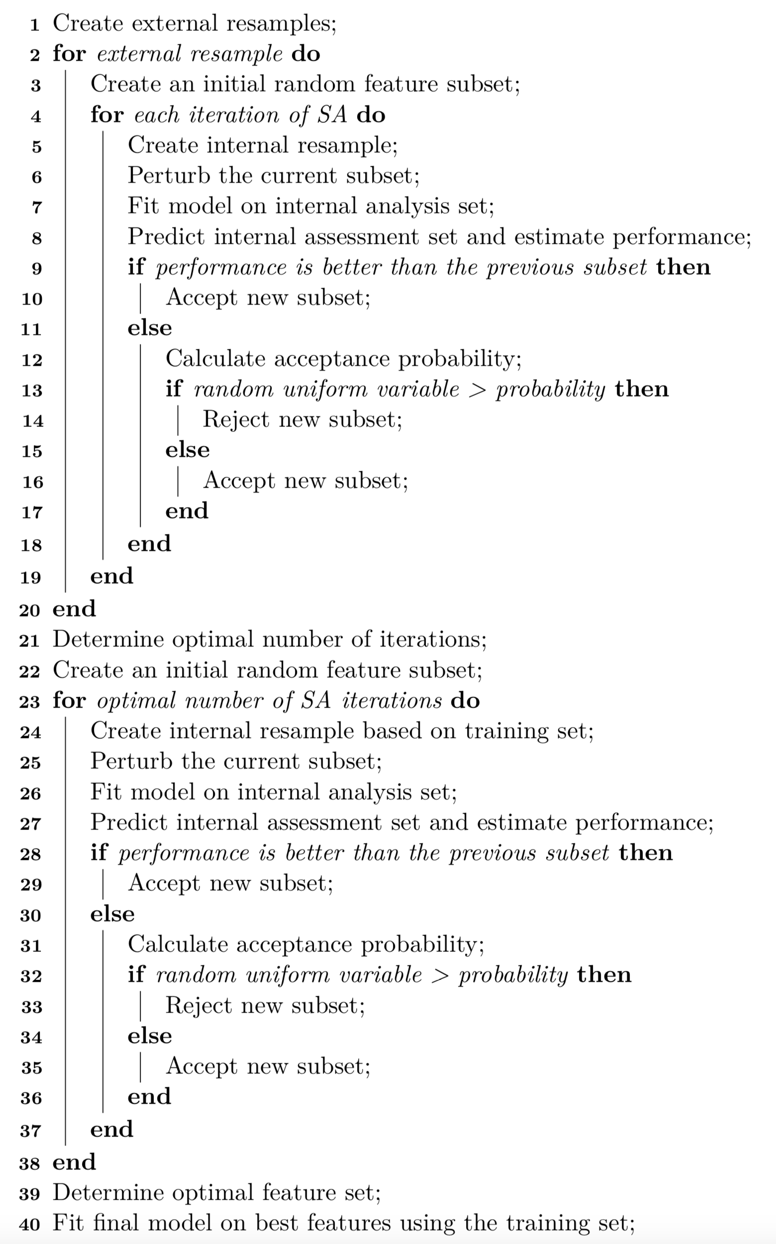
An external resampling procedure should be used to determine how many iterations of the search are appropriate. This would average the assessment set predictions across all resamples to determine how long the search should proceed when it is directly applied to the entire training set. Basically, the number of iterations is a tuning parameter
A good way to do this is with 10 fold cross validation. The author recommends separating the external resample into train and evaluation.

Figure 12.2: A diagram of external and internal cross-validation for global search.
the internal resamples guide the subset selection process
the external resamples help tune the number of search iterations to use.
The resampling selection procedure is as follows:
12.2.2 12.2.2 Application to Modeling the OkCupid Data
To put simulated annealing in practice, again the OkCupid data is used. The area under the ROC curve is used to optimize the models and to find the optimal number of SA iterations.

Figure 12.3: Internal performance profile for naive Bayes models selected via simulated annealing for each external resample.
Then both external and internal performance estimates are compared by using rank correlation. The average rank correlation between the two sets of ROC statistics is 0.622 with a range of (0.43, 0.85). This indicates fairly good consistency. While there is substantial variability in these values, the number of variables selected at those points in the process are more precise; the average was 56 predictors with a range of (49, 64)

Figure 12.4: Performance profile for naive Bayes models selected via simulated annealing where a random 50 percent of the features were seeded into the initial subset.
For the final search, what was done inside of the external resamples is repeated to measure ROC and sample size.

Figure 12.5: Trends for the final SA search using the entire training set and a 10 percent internal validation set.
During this final search, the iteration with the best area under the ROC curve (0.837) was 356 where 63 predictors were used.
12.2.3 12.2.3 Examining Changes in Performance
In order to measure the importance of features a t-test for equality can be conducted to tease out the important variables from all of the subsets.
12.2.4 12.2.4 Grouped Qualitative Predictors Versus Indicator Variables
Using categorical features (one hot encoded) has the potential to dramatically increase computation time and slightly decrease the performance (not by much)

Figure 12.6: Results when qualitative variables are decomposed into individual predictors.
12.2.5 12.2.5 The Effect of the Initial Subset
Figure 12.7 shows the smoothed subset sizes for each external resample colored by the different initial percentages. In many instances, the three configurations converged to a subset size that was about half of the total number of possible predictors (although a few showed minimal change overall).

Figure 12.7: Resampling trends across iterations for different initial feature subset sizes. These results were achieved using simulated annealing applied to the OkCupid data.
In terms of performance, the areas under the ROC curves for the three sets were 0.805 (10%), 0.799 (50%), and 0.804 (90%).