1.3 A model with two predictors
data(segmentationData)This example uses segmentationData. Data originates from an experiment from Hill et al. (2007), a study on “Impact of Image Segmentation on High-Content Screening Data Quality for SK-BR-3 Cells.” BMC Bioinformatics.
The data set includes a Case vector containing Train and Test variables, with a total of 61 different vectors, about cellular structures and morphology.
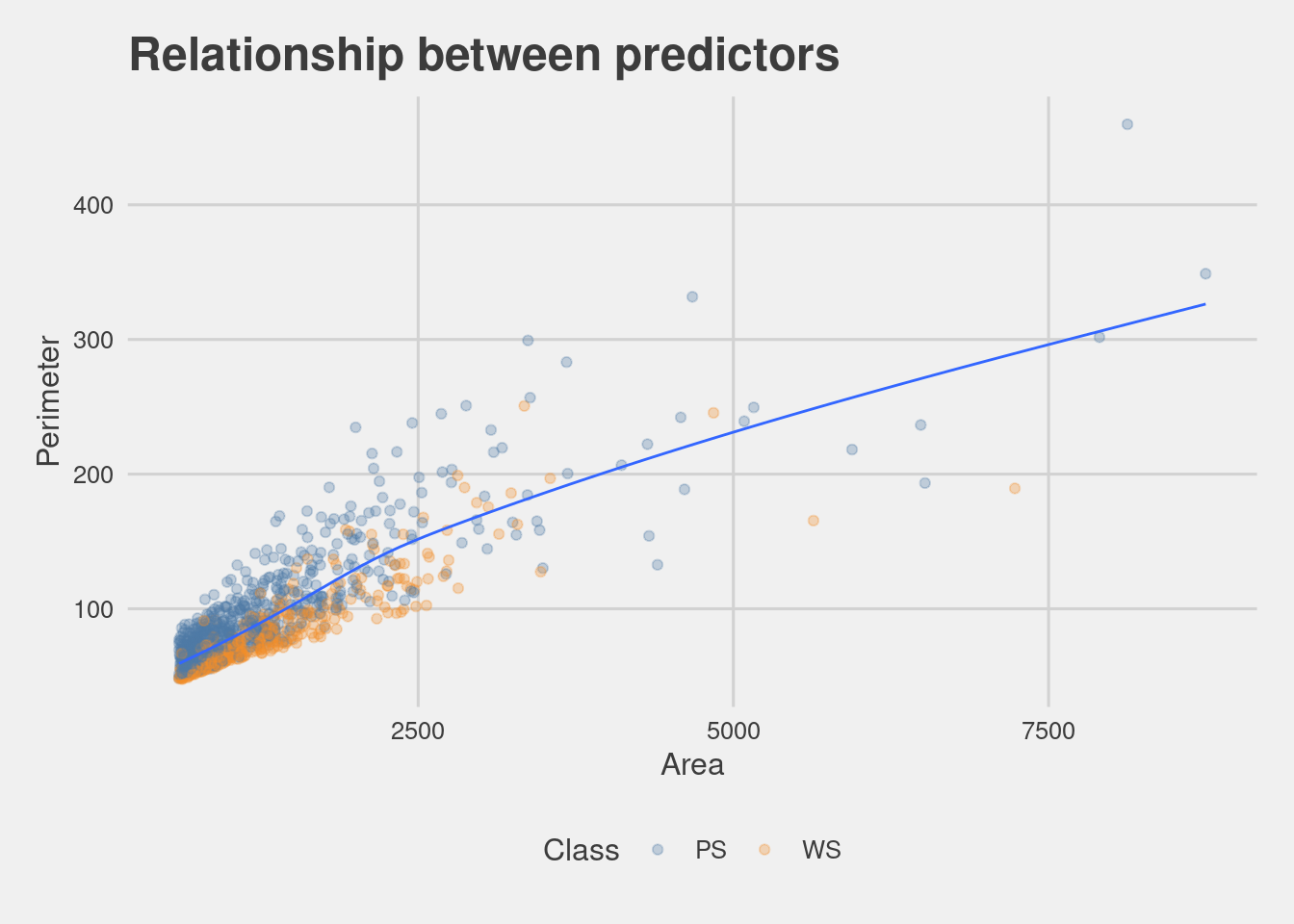
Selected for this first example are two predictors: EqSphereAreaCh1 and PerimCh1. The objective is to predict shape parameters of poorly-segmented (PS) and well-segmented (WS) cells from the Class variable.
This is the full list of variables in the set.
##  [1] "Cell"                    "Case"
##  [3] "Class"                   "AngleCh1"
##  [5] "AreaCh1"                 "AvgIntenCh1"
##  [7] "AvgIntenCh2"             "AvgIntenCh3"
##  [9] "AvgIntenCh4"             "ConvexHullAreaRatioCh1"
## [11] "ConvexHullPerimRatioCh1" "DiffIntenDensityCh1"
## [13] "DiffIntenDensityCh3"     "DiffIntenDensityCh4"
## [15] "EntropyIntenCh1"         "EntropyIntenCh3"
## [17] "EntropyIntenCh4"         "EqCircDiamCh1"
## [19] "EqEllipseLWRCh1"         "EqEllipseOblateVolCh1"
## [21] "EqEllipseProlateVolCh1"  "EqSphereAreaCh1"
## [23] "EqSphereVolCh1"          "FiberAlign2Ch3"
## [25] "FiberAlign2Ch4"          "FiberLengthCh1"
## [27] "FiberWidthCh1"           "IntenCoocASMCh3"
## [29] "IntenCoocASMCh4"         "IntenCoocContrastCh3"
## [31] "IntenCoocContrastCh4"    "IntenCoocEntropyCh3"
## [33] "IntenCoocEntropyCh4"     "IntenCoocMaxCh3"
## [35] "IntenCoocMaxCh4"         "KurtIntenCh1"
## [37] "KurtIntenCh3"            "KurtIntenCh4"
## [39] "LengthCh1"               "NeighborAvgDistCh1"
## [41] "NeighborMinDistCh1"      "NeighborVarDistCh1"
## [43] "PerimCh1"                "ShapeBFRCh1"
## [45] "ShapeLWRCh1"             "ShapeP2ACh1"
## [47] "SkewIntenCh1"            "SkewIntenCh3"
## [49] "SkewIntenCh4"            "SpotFiberCountCh3"
## [51] "SpotFiberCountCh4"       "TotalIntenCh1"
## [53] "TotalIntenCh2"           "TotalIntenCh3"
## [55] "TotalIntenCh4"           "VarIntenCh1"
## [57] "VarIntenCh3"             "VarIntenCh4"
## [59] "WidthCh1"                "XCentroid"
## [61] "YCentroid"
## [1] 2019 61Parsimony:
##   Class     Area Perimeter
## 1    PS 3278.726 154.89876
## 2    WS 1727.410  84.56460
## 3    PS 1194.932 101.09107
## 4    WS 1027.222  68.71062
## 5    PS 1035.608  73.40559
## 6    PS 1433.918  79.47569
The dataset is already split between training and test sets, all that is to be added is cross-validation on the training set.
set.seed(2222)
folds <- vfold_cv(train, v = 10)
A first visualization of the relationship between the two predictors.
Check for Class imbalance of the response variable
This would be the first level transformation of the response, this type of transformation is considered a structural transformation, we will see more about it later in the book.
             PS     WS
tb_class 636.00 373.00
pr_class   0.63   0.37
up_samp_ws <- pr_class[2]Recipes
library(themis)

log_rec_natural_units <- recipe(Class ~ Area + Perimeter, data = train) %>%
  step_upsample(Class, over_ratio = up_samp_ws)

log_rec_inverse_units <- recipe(Class ~ Area + Perimeter, data = train) %>%
  step_upsample(Class, over_ratio = up_samp_ws) %>%
  step_BoxCox(all_numeric())
Workflow
logistic_reg_glm_spec <-
  logistic_reg() %>%
  set_engine('glm')


log_wfl_natural_units <- workflow() %>%
  add_model(logistic_reg_glm_spec) %>%
  add_recipe(log_rec_natural_units)


log_fit_natural_units <- log_wfl_natural_units %>%
  fit(train)

log_fit_natural_units %>%
  extract_fit_parsnip() %>%
  tidy()
# A tibble: 3 × 5
term estimate std.error statistic p.value
<chr> <dbl> <dbl> <dbl> <dbl>
1 (Intercept) 1.58 0.248 6.36 1.99e-10
2 Area 0.00301 0.000281 10.7 8.95e-27
3 Perimeter -0.0682 0.00604 -11.3 1.47e-29Prediction
with_pred_natural_units <- log_fit_natural_units %>%
  augment(test)

with_pred_natural_units %>% head
# A tibble: 6 × 6
Class Area Perimeter .pred_class .pred_PS .pred_WS
<fct> <dbl> <dbl> <fct> <dbl> <dbl>
1 PS 742. 68.8 PS 0.705 0.295
2 PS 1140. 86.5 PS 0.707 0.293
3 WS 692. 49.5 WS 0.429 0.571
4 WS 709. 50.4 WS 0.431 0.569
5 PS 1006. 89.9 PS 0.820 0.180
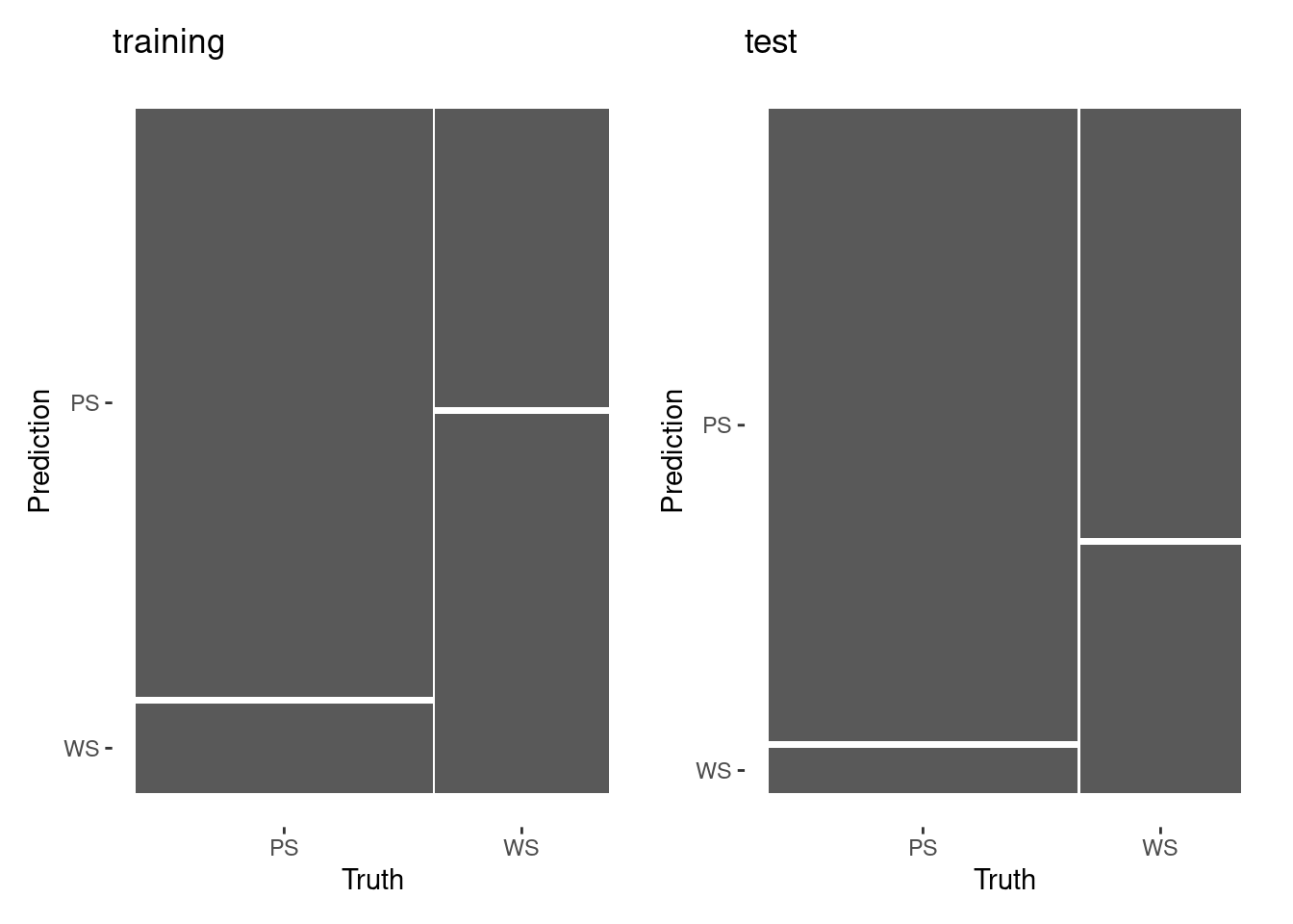
6 WS 1983. 112. PS 0.516 0.484Confusion Matrics
Roc Curve
with_pred_natural_units  %>%
  roc_curve(Class,.pred_PS) %>%
  mutate(Format = "Natural Units") %>%
  ggplot(aes(1 - specificity, sensitivity))+
  geom_line(aes(color = .threshold), size = 1)+
  geom_abline(linetype = "dashed", size = 1, color = "gray") +
  scale_colour_continuous()+
  theme_fivethirtyeight() +
  theme(axis.title = element_text())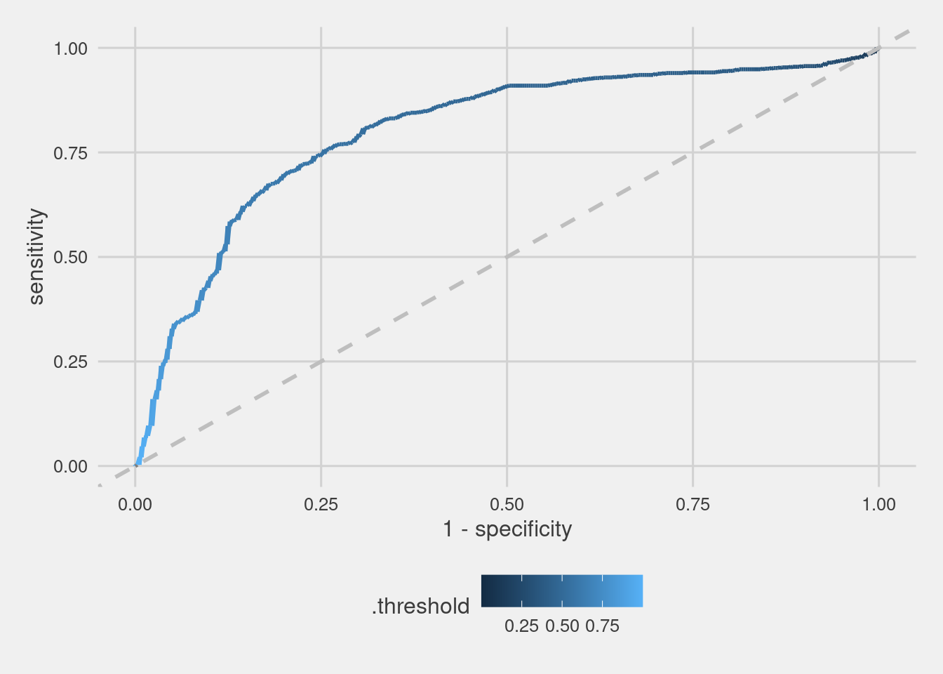
Workflow set
Let’s compare the two transformations with a workflow_set():
full_workflow <- workflow_set(
  models = list(logitstic = logistic_reg_glm_spec),
  preproc = list(natural_units = log_rec_natural_units,
                 inverse_units = log_rec_inverse_units))

system.time(
  grid_results <- full_workflow %>%
    workflow_map(
      seed = 1503,
      resamples = folds,
      grid = 25,
      control = control_grid(
        save_pred = TRUE,
        parallel_over = "everything",
        save_workflow = TRUE),
      verbose = TRUE)
  )
user system elapsed
6.748 0.048 6.797 grid_results# A workflow set/tibble: 2 × 4
wflow_id info option result
<chr> <list> <list> <list>
1 natural_units_logitstic <tibble [1 × 4]> <opts[3]> <rsmp[+]>
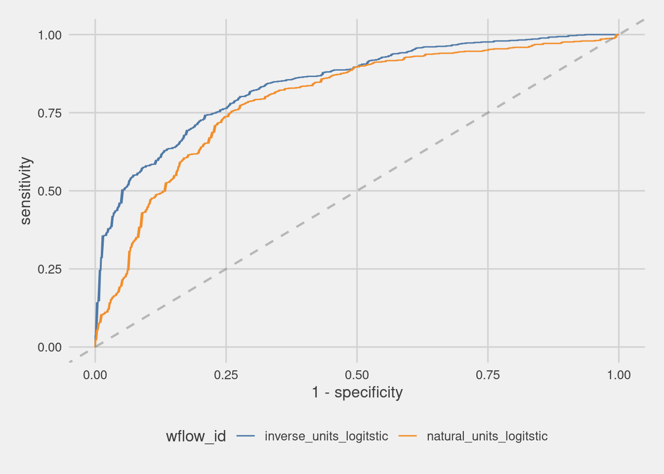
2 inverse_units_logitstic <tibble [1 × 4]> <opts[3]> <rsmp[+]>Roc curves for two different recipes
roc <- grid_results %>%
  unnest(result) %>%
  unnest(.predictions) %>%
  select(wflow_id, .pred_PS, .pred_WS, .pred_class, Class) %>%
  group_by(wflow_id) %>%
  roc_curve(Class, .pred_PS)

roc_curves <- roc %>%
  ggplot(
    aes(x = 1 - specificity, y = sensitivity, group = wflow_id, color = wflow_id)
  ) +
  geom_line(size = 0.5) +
  geom_abline(lty = 2, alpha = 0.5, color = "gray50", size = 0.8)+
  scale_color_tableau()+
  theme_fivethirtyeight()+
  theme(axis.title = element_text())
roc_curves