3.4 Relationship between variables: Linear models and correlation

Examples:

1. want to know about expression of a particular gene in liver in relation to the dosage of a drug that patient receives
2. DNA methylation of a certain locus in the genome in relation to the age of the sample donor.
3. relationship between histone modifications and gene expression.

$$Y=\beta_0+\beta_1X+\epsilon$$ Approximation of the response:

$$Y\sim\beta_0+\beta_1X$$ Estimation of the coefficients:

$$Y=\hat{\beta_0}+\hat{\beta_1}X$$

More than one predictor:

$$Y=\beta_0+\beta_1X_1+\beta_2X_2+\epsilon$$ $$Y=\beta_0+\beta_1X_1+\beta_2X_2+\beta_3X_3+...+\beta_nX_n+\epsilon$$

$$Y=\begin{bmatrix} 1 & X_{1,1} & X_{1,2}\\ 1 & X_{2,1} & X_{2,2}\\ 1 & X_{3,1} & X_{3,2}\\ 1 & X_{4,1} & X_{4,2} \end{bmatrix}\begin{bmatrix} \beta_0 \\ \beta_1 \\ \beta_2 \end{bmatrix}+\begin{bmatrix} \epsilon_1 \\ \epsilon_2 \\ \epsilon_3\\ \epsilon_0 \end{bmatrix}$$

$$Y_1=\beta_0+\beta_1X_{1,1}+\beta_2X_{1,2}+\epsilon_1$$ $$Y_1=\beta_0+\beta_1X_{2,1}+\beta_2X_{2,2}+\epsilon_2$$ $$Y_1=\beta_0+\beta_1X_{3,1}+\beta_2X_{3,2}+\epsilon_3$$ $$Y_1=\beta_0+\beta_1X_{4,1}+\beta_2X_{4,2}+\epsilon_4$$

$$Y=X\beta+\epsilon$$

3.4.1 The cost or loss function approach

Minimize the residuals: optimization procedure

$$min\sum{(y_i=(\beta_0+\beta_1x_1))^2}$$

The “gradient descent” algorithm”

1. Pick a random starting point, random $\beta$ values.

2. Take the partial derivatives of the cost function to see which direction is the way to go in the cost function.

3. Take a step toward the direction that minimizes the cost function.

   • Step size is a parameter to choose, there are many variants.

4. Repeat step 2,3 until convergence.

The algorithm usually converges to optimum $\beta$ values.

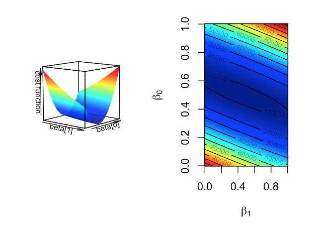
Figure 3.1: Cost function landscape for linear regression with changing beta values. The optimization process tries to find the lowest point in this landscape by implementing a strategy for updating beta values toward the lowest point in the landscape.

3.4.2 The “maximum likelihood” approach

• The response variable $y_i$ follows a normal distribution with mean $\beta_0+\beta_1x_i$ and variance $s^2$.

• Find $\beta_0$ and $\beta_1$ that maximizes the probability of observing all the response variables in the dataset given the explanatory variables.

• constant variance $s^2$, estimation of the variance of the population $\sigma^2$

$$s^2=\frac{\sum{\epsilon_i}}{n-2}$$ Probability:

$$P(y_i)=\frac{1}{s\sqrt{2\pi}}e^{-\frac{1}{2}(\frac{y_i-(\beta_0+\beta_1x_i)}{s})^2}$$

Likelihood function:

$$L=P(y_1)P(y_2)P(y_3)..P(y_n)=\prod_{i=1}^{n}{P_i}$$

The log:

$$ln(L)=-nln(s\sqrt{2\pi})-\frac{1}{2s^2}\sum_{i=1}{n}{(y_i-(\beta_0+\beta_1x_i))^2}$$ the negative of the cost function: $$-\frac{1}{2s^2}\sum_{i=1}{n}{(y_i-(\beta_0+\beta_1x_i))^2}$$ to optimize this function we would need to take the derivative of the function with respect to the parameters.

3.4.3 Linear algebra and closed-form solution to linear regression

$$\epsilon_i=Y_i-(\beta_0+\beta_1x_i)$$

$$\sum{\epsilon_i^2}=\epsilon^T\epsilon=(Y-\beta X)^T(Y-\beta X)$$ $$= Y^TY-(2\beta^T Y + \beta^T X^T X\beta)$$

$$\hat{\beta}=(X^T X)^{-1}X^T Y$$

$$\hat{\beta_1}=\frac{\sum{(x_i-\bar{X})(y_i-\bar{Y})}}{\sum{(x_i-\bar{X})^2}}$$

$$\hat{\beta_0}=\bar{Y}-\hat{\beta_1}\bar{X}$$

# set random number seed, so that the random numbers from the text
# is the same when you run the code.
set.seed(32)

# get 50 X values between 1 and 100
x = runif(50,1,100)

# set b0,b1 and variance (sigma)
b0 = 10
b1 = 2
sigma = 20
# simulate error terms from normal distribution
eps = rnorm(50,0,sigma)
# get y values from the linear equation and addition of error terms
y = b0 + b1*x+ eps

mod1=lm(y~x)

# plot the data points
plot(x,y,pch=20,
     ylab="Gene Expression",xlab="Histone modification score")
# plot the linear fit
abline(mod1,col="blue")

3.4.4 How to estimate the error of the coefficients

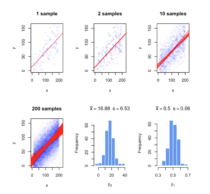
Figure 3.2: Regression coefficients vary with every random sample. The figure illustrates the variability of regression coefficients when regression is done using a sample of data points. Histograms depict this variability for b0 and b1 coefficients.

The calculation of the Residual Standard Error (RSE)

$$s=RSE$$

mod1=lm(y~x)
summary(mod1)

## 
## Call:
## lm(formula = y ~ x)
## 
## Residuals:
##    Min     1Q Median     3Q    Max 
## -38.50 -12.62   1.66  14.26  37.20 
## 
## Coefficients:
##             Estimate Std. Error t value Pr(>|t|)    
## (Intercept)  0.40951    6.43208   0.064     0.95    
## x            2.08742    0.09775  21.355   <2e-16 ***
## ---
## Signif. codes:  0 '***' 0.001 '**' 0.01 '*' 0.05 '.' 0.1 ' ' 1
## 
## Residual standard error: 16.96 on 48 degrees of freedom
## Multiple R-squared:  0.9048, Adjusted R-squared:  0.9028 
## F-statistic:   456 on 1 and 48 DF,  p-value: < 2.2e-16

# get confidence intervals 
confint(mod1)

##                  2.5 %    97.5 %
## (Intercept) -12.523065 13.342076
## x             1.890882  2.283952

# pull out coefficients from the model
coef(mod1)

## (Intercept)           x 
##   0.4095054   2.0874167

3.4.5 Accuracy of the model

$$s=RSE=\sqrt{\frac{\sum{(y_i-\hat{Y_i})^2}}{n-p}}=\sqrt{\frac{RSS}{n-p}}$$

$$R^2=1-\frac{RSS}{TSS}=\frac{TSS-RSS}{TSS}=1-\frac{RSS}{TSS}$$

$$r_{xy}=\frac{cov(X,Y)}{\sigma_x\sigma_y}=\frac{\sum_{i=1}^n{(x_i-\bar{x})(y_i-\bar{y})}}{\sqrt{\sum_{i=1}^n{(x_i-\bar{x})^2\sum_{i=1}^n{(y_i-\bar{y})^2}}}}$$

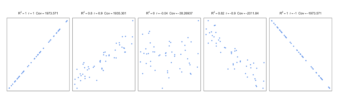
Figure 3.3: Correlation and covariance for different scatter plots.

$$H_0:\beta_1=\beta_2=\beta_3=...=\beta_p=0$$

$$H_1:\text{at least one}\beta_1\neq0$$

The F-statistic for a linear model

$$F=\frac{(TSS-RSS)/(p-1)}{RSS/(n-p)}=\frac{(TSS-RSS)/(p-1)}{RSE}\sim{F(p-1,n-p)}$$

3.4.6 Regression with categorical variables

set.seed(100)
gene1=rnorm(30,mean=4,sd=2)
gene2=rnorm(30,mean=2,sd=2)
gene.df=data.frame(exp=c(gene1,gene2),
                  group=c( rep(1,30),rep(0,30) ) )

mod2=lm(exp~group,data=gene.df)
summary(mod2)

## 
## Call:
## lm(formula = exp ~ group, data = gene.df)
## 
## Residuals:
##     Min      1Q  Median      3Q     Max 
## -4.7290 -1.0664  0.0122  1.3840  4.5629 
## 
## Coefficients:
##             Estimate Std. Error t value Pr(>|t|)    
## (Intercept)   2.1851     0.3517   6.214 6.04e-08 ***
## group         1.8726     0.4973   3.765 0.000391 ***
## ---
## Signif. codes:  0 '***' 0.001 '**' 0.01 '*' 0.05 '.' 0.1 ' ' 1
## 
## Residual standard error: 1.926 on 58 degrees of freedom
## Multiple R-squared:  0.1964, Adjusted R-squared:  0.1826 
## F-statistic: 14.18 on 1 and 58 DF,  p-value: 0.0003905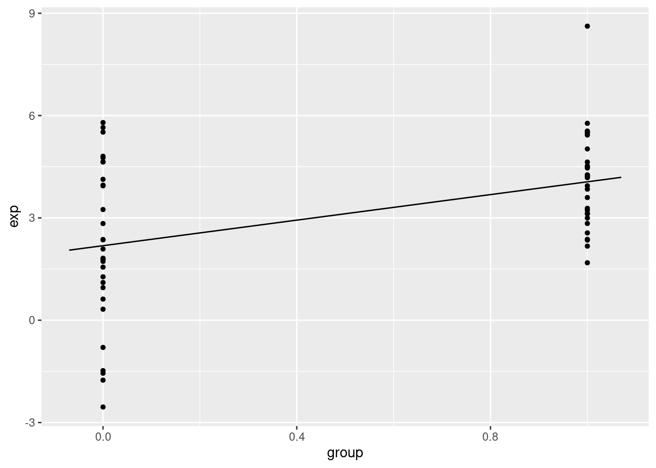

require(mosaic)
plotModel(mod2)

gene.df=data.frame(exp=c(gene1,gene2,gene2),
                  group=c( rep("A",30),rep("B",30),rep("C",30) ) 
                  )

mod3=lm(exp~group,data=gene.df)
summary(mod3)

## 
## Call:
## lm(formula = exp ~ group, data = gene.df)
## 
## Residuals:
##     Min      1Q  Median      3Q     Max 
## -4.7290 -1.0793 -0.0976  1.4844  4.5629 
## 
## Coefficients:
##             Estimate Std. Error t value Pr(>|t|)    
## (Intercept)   4.0577     0.3781  10.731  < 2e-16 ***
## groupB       -1.8726     0.5348  -3.502 0.000732 ***
## groupC       -1.8726     0.5348  -3.502 0.000732 ***
## ---
## Signif. codes:  0 '***' 0.001 '**' 0.01 '*' 0.05 '.' 0.1 ' ' 1
## 
## Residual standard error: 2.071 on 87 degrees of freedom
## Multiple R-squared:  0.1582, Adjusted R-squared:  0.1388 
## F-statistic: 8.174 on 2 and 87 DF,  p-value: 0.0005582

3.4.7 Regression pitfalls

• Non-linearity
• Correlation of explanatory variables
• Correlation of error terms
• Non-constant variance of error terms
• Outliers and high leverage points