8.3 Exploratory analysis
Check for similarity of biological replicates.
- clustering
- PCA
- Correlation plots
(see also Chapter 4)
Clustering possible with different packages/functions (stats::heatmap, pheatmap, ComplexHeatmap).
#compute the variance of each gene across samples
V <- apply(tpm, 1, var)
#sort the results by variance in decreasing order
#and select the top 100 genes
selectedGenes <- names(V[order(V, decreasing = T)][1:100])library(pheatmap)
colData <- read.table(coldata_file, header = T, sep = '\t',
stringsAsFactors = TRUE)
pheatmap(tpm[selectedGenes,], scale = 'row',
show_rownames = FALSE,
annotation_col = colData)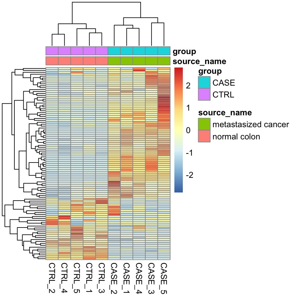
hierarchical clustering
PCA
library(stats)
library(ggplot2)
#transpose the matrix
M <- t(tpm[selectedGenes,])
# transform the counts to log2 scale
M <- log2(M + 1)
#compute PCA
pcaResults <- prcomp(M)

#plot PCA results making use of ggplot2's autoplot function
#ggfortify is needed to let ggplot2 know about PCA data structure.
autoplot(pcaResults, data = colData, colour = 'group')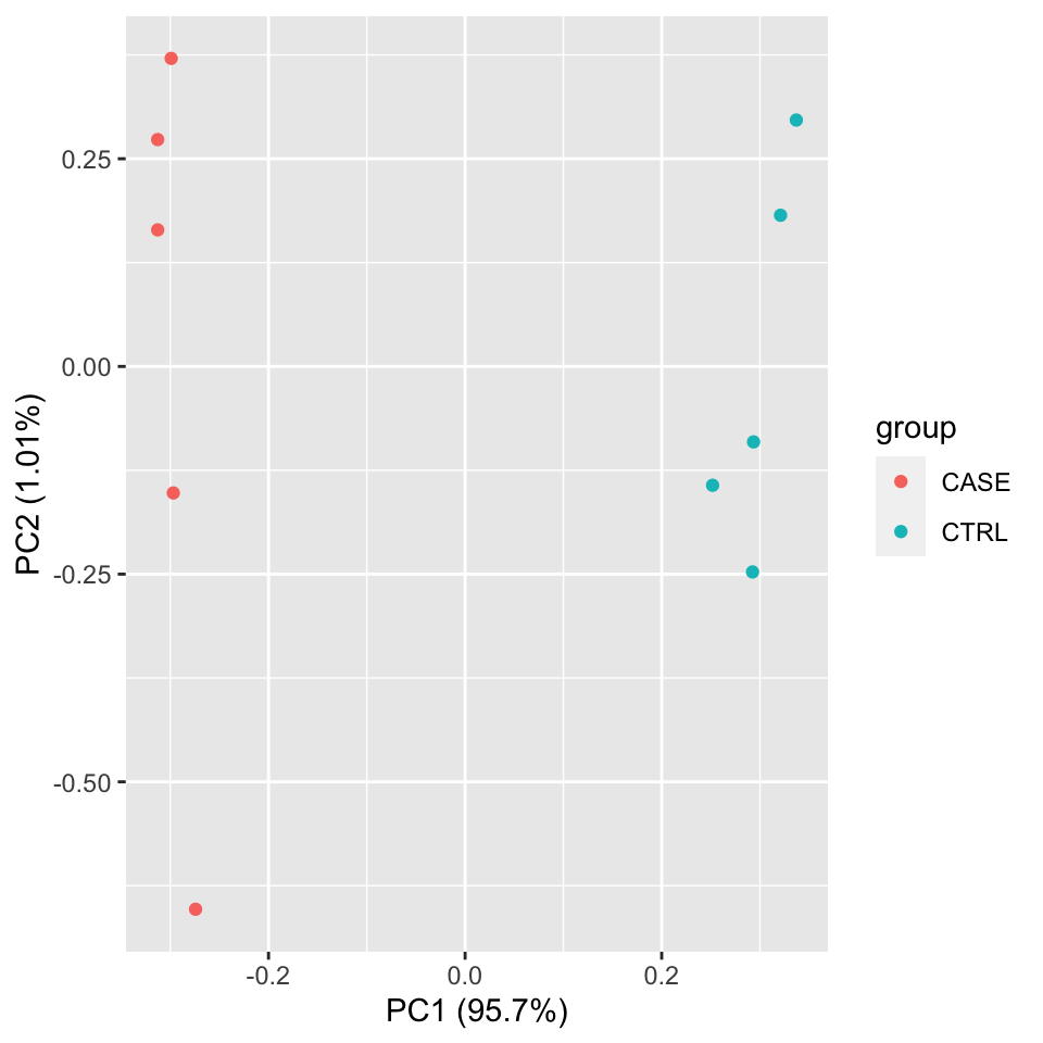
PCA
Correlation plots
library(pheatmap)
# split the clusters into two based on the clustering similarity
pheatmap(correlationMatrix,
         annotation_col = colData,
         cutree_cols = 2)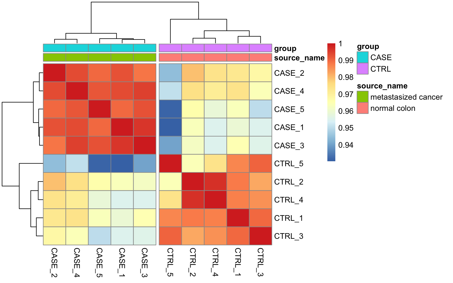
Correlation plot