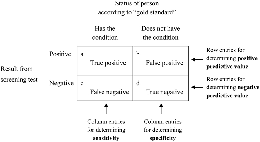
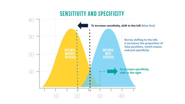
5.5 Precision, Specificity, and Sensitivity

# get k-NN prediction on the training data itself, with k=5
knnFit=knn3(x=training[,-1], # training set
            y=training[,1], # training set class labels
            k=5)

# predictions on the training set
trainPred=predict(knnFit,training[,-1],type="class")

# compare the predicted labels to real labels
# get different performance metrics
confusionMatrix(data=training[,1],reference=trainPred)

## Confusion Matrix and Statistics
## 
##           Reference
## Prediction CIMP noCIMP
##     CIMP     62      3
##     noCIMP   13     52
##                                          
##                Accuracy : 0.8769         
##                  95% CI : (0.8078, 0.928)
##     No Information Rate : 0.5769         
##     P-Value [Acc > NIR] : 9.216e-14      
##                                          
##                   Kappa : 0.7538         
##                                          
##  Mcnemar's Test P-Value : 0.02445        
##                                          
##             Sensitivity : 0.8267         
##             Specificity : 0.9455         
##          Pos Pred Value : 0.9538         
##          Neg Pred Value : 0.8000         
##              Prevalence : 0.5769         
##          Detection Rate : 0.4769         
##    Detection Prevalence : 0.5000         
##       Balanced Accuracy : 0.8861         
##                                          
##        'Positive' Class : CIMP           
## 

# predictions on the test set, return class labels
testPred=predict(knnFit,testing[,-1],type="class")

# compare the predicted labels to real labels
# get different performance metrics
confusionMatrix(data=testing[,1],reference=testPred)

## Confusion Matrix and Statistics
## 
##           Reference
## Prediction CIMP noCIMP
##     CIMP     25      2
##     noCIMP    6     21
##                                           
##                Accuracy : 0.8519          
##                  95% CI : (0.7288, 0.9338)
##     No Information Rate : 0.5741          
##     P-Value [Acc > NIR] : 1.182e-05       
##                                           
##                   Kappa : 0.7037          
##                                           
##  Mcnemar's Test P-Value : 0.2888          
##                                           
##             Sensitivity : 0.8065          
##             Specificity : 0.9130          
##          Pos Pred Value : 0.9259          
##          Neg Pred Value : 0.7778          
##              Prevalence : 0.5741          
##          Detection Rate : 0.4630          
##    Detection Prevalence : 0.5000          
##       Balanced Accuracy : 0.8597          
##                                           
##        'Positive' Class : CIMP            
## 

library(pROC)

## Type 'citation("pROC")' for a citation.

## 
## Attaching package: 'pROC'

## The following objects are masked from 'package:mosaic':
## 
##     cov, var

## The following objects are masked from 'package:stats':
## 
##     cov, smooth, var

# get k-NN class probabilities
# prediction probabilities on the test set
testProbs=predict(knnFit,testing[,-1])

# get the roc curve
rocCurve <- pROC::roc(response = testing[,1],
                predictor = testProbs[,1],
              ## This function assumes that the second
              ## class is the class of interest, so we
              ## reverse the labels.
              levels = rev(levels(testing[,1])))

## Setting direction: controls < cases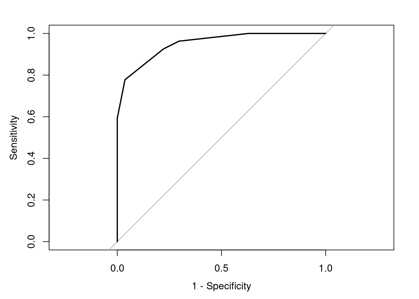

# plot the curve
plot(rocCurve, legacy.axes = TRUE)

# return area under the curve
pROC::auc(rocCurve)

## Area under the curve: 0.9506