15.1 Theory

Tobler’s first law of geography

“Everything is related to everything else, but near things are more related than distant things”

Recalling John Snow's belief that the cause of cholera was water-borne.

In summary, spatial autocorrelation is the degree to which the values of a variable in one location are correlated with the values of the same variable in neighboring locations.

15.1.1 Moran’s I

Moran's Test \(I\) helps us understand if this similarity (nearby locations are more similar to each other than to distant locations) is statistically significant or just due to chance.

It will provide a p-value, if the p-value is low (typically less than 0.05), there is significant spatial autocorrelation in the data, or a non-random pattern.

\[I=\frac{n\sum_{(2)}{w_{ij}z_iz_j}}{S_0\sum_{i=1}^n{z_i^2}}\]

\(z_i=x_i-\bar{x}\)
\(\bar{x}=\sum_{i=1}^n{x_i/n}\)
\(w_{ij}=\text{spatial weights}\)
\(S_0= \sum_{(2)}{w_{ij}}\)

library(spdep) |> suppressPackageStartupMessages()
# library(parallel)

glance_htest <- function(ht) c(ht$estimate, 
    "Std deviate" = unname(ht$statistic), 
    "p.value" = unname(ht$p.value))

15.1.2 Case Study: Polish election data

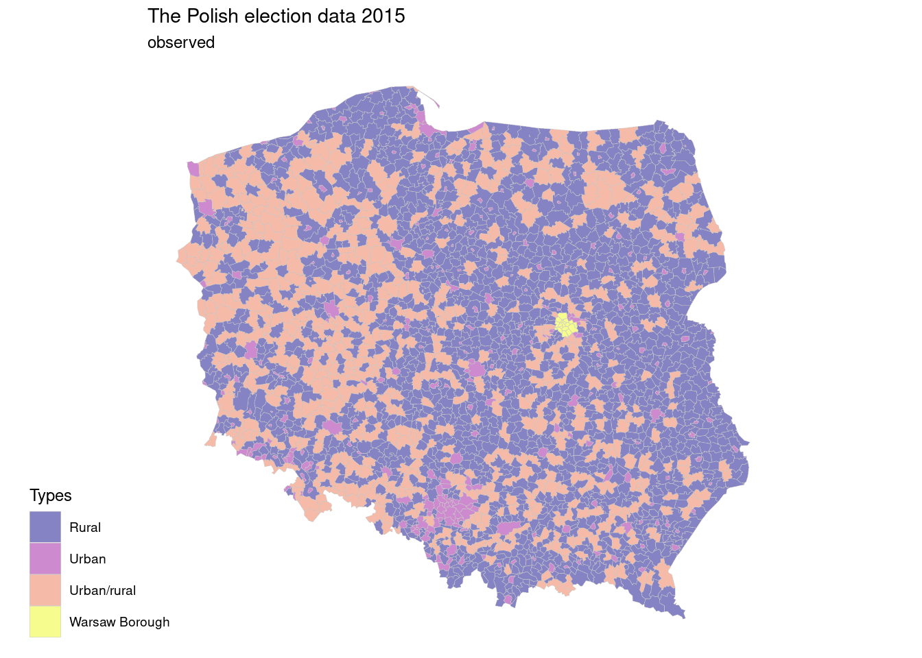
The Polish election data 2015, pol_pres15, shows results of elections by type of area.

data(pol_pres15, package = "spDataLarge")
pol_pres15 %>%
  dplyr::select(types,I_turnout) %>%
  head

## Simple feature collection with 6 features and 2 fields
## Geometry type: MULTIPOLYGON
## Dimension:     XY
## Bounding box:  xmin: 235157.1 ymin: 366913.3 xmax: 281431.7 ymax: 413016.6
## Projected CRS: ETRS89 / Poland CS92
##         types I_turnout                       geometry
## 1       Urban 0.4768987 MULTIPOLYGON (((261089.5 38...
## 2       Rural 0.4338417 MULTIPOLYGON (((254150 3837...
## 3       Rural 0.4280679 MULTIPOLYGON (((275346 3846...
## 4 Urban/rural 0.3739735 MULTIPOLYGON (((251769.8 37...
## 5       Rural 0.4066215 MULTIPOLYGON (((263423.9 40...
## 6       Rural 0.3853731 MULTIPOLYGON (((267030.7 38...

library(tidyverse)
map1 <- ggplot(pol_pres15) +
  geom_sf(aes(geometry=geometry,fill=types),
          linewidth=0.1,
          color="grey80",
          alpha=0.5)+
  scale_fill_viridis_d(option = "C",direction = 1)+
  labs(title="The Polish election data 2015",
       subtitle = "observed",
       fill="Types")+
  ggthemes::theme_map()+
  theme(legend.position = c(-0.2,0))
map1

?st_make_valid

pol_pres15 <- st_make_valid(pol_pres15)

map1

15.1.2.1 Moran’s I components

Construct neighbours list from polygon list based on regions with contiguous boundaries.

?poly2nb

nb_q <- pol_pres15 |> 
  poly2nb(queen = TRUE)
nb_q

## Neighbour list object:
## Number of regions: 2495 
## Number of nonzero links: 14242 
## Percentage nonzero weights: 0.2287862 
## Average number of links: 5.708216

Spatial weights for neighbours lists function adds a weights list with values given by the coding scheme style chosen. B is the basic binary coding.

?nb2listw

lw_q_B <- nb_q |> 
    nb2listw(style = "B") 
lw_q_B

## Characteristics of weights list object:
## Neighbour list object:
## Number of regions: 2495 
## Number of nonzero links: 14242 
## Percentage nonzero weights: 0.2287862 
## Average number of links: 5.708216 
## 
## Weights style: B 
## Weights constants summary:
##      n      nn    S0    S1     S2
## B 2495 6225025 14242 28484 357280

15.1.2.2 Hypothesis testing

For testing for autocorrelation we first build a random Normal, rnorm distribution of values based on the number of observations.

set.seed(1)
x <- pol_pres15 |> 
    nrow() |> 
    rnorm()

Then apply the Moran’s I test for spatial autocorrelation to check the randomness of data.

?moran.test

\[\left\{\begin{matrix} H_0 & p\leq0.05\\ H_a& p>0.05 \end{matrix}\right. \]

If the p-value is low (typically less than 0.05), it suggests that there is significant spatial autocorrelation in the data, indicating a non-random pattern.

x |> 
    moran.test(lw_q_B, #Spatial weights  
               randomisation = FALSE,
               alternative = "two.sided")

## 
##  Moran I test under normality
## 
## data:  x  
## weights: lw_q_B    
## 
## Moran I statistic standard deviate = -0.36932, p-value = 0.7119
## alternative hypothesis: two.sided
## sample estimates:
## Moran I statistic       Expectation          Variance 
##     -0.0047715202     -0.0004009623      0.0001400449

Now see what happens if we use our data and add a gentle trend.

library(sf)
coords <- pol_pres15 |> 
    st_geometry() |> # select the geometry
    st_centroid(of_largest_polygon = TRUE)

Adding a gentle trend things changed:

beta <- 0.0015
t <- coords |> 
    st_coordinates() |> # transform the geometry into lat and long
    subset(select = 1, drop = TRUE) |> 
    (function(x) x/1000)()

This is our new data:

 (x + beta * t)

x_t <- (x + beta * t) 

x_t |> 
    moran.test(lw_q_B, 
               randomisation = FALSE,
               alternative = "two.sided")

## 
##  Moran I test under normality
## 
## data:  x_t  
## weights: lw_q_B    
## 
## Moran I statistic standard deviate = 3.7015, p-value = 0.0002143
## alternative hypothesis: two.sided
## sample estimates:
## Moran I statistic       Expectation          Variance 
##      0.0434026880     -0.0004009623      0.0001400449

15.1.3 Test the residuals

Here we apply the Moran’s I test for residual spatial autocorrelation to a linear model specification.

?lm.morantest

lm(x_t ~ t) |> 
    lm.morantest(lw_q_B, 
                 alternative = "two.sided")

## 
##  Global Moran I for regression residuals
## 
## data:  
## model: lm(formula = x_t ~ t)
## weights: lw_q_B
## 
## Moran I statistic standard deviate = -0.33731, p-value = 0.7359
## alternative hypothesis: two.sided
## sample estimates:
## Observed Moran I      Expectation         Variance 
##    -0.0047772213    -0.0007891850     0.0001397877