7.4 Spatial Joins
- The concepts of “left”, “right”, “inner”, or “full” joins remain
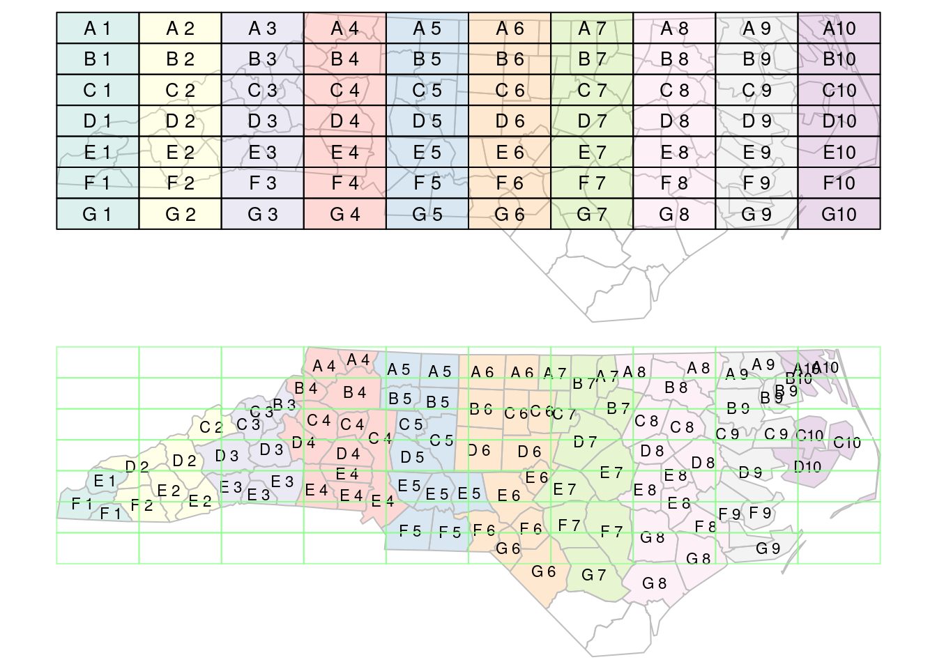
When using spatial joins, each record may have several matched records … A way to reduce this complexity may be to select from the matching records the one with the largest overlap with the target geometry.
Loading shapefile and grid
system.file("shape/nc.shp", package="sf") |>
    read_sf() |>
    st_transform('EPSG:2264') -> nc
gr <- st_sf(
         label = apply(expand.grid(1:10, LETTERS[10:1])[,2:1], 1, paste0, collapse = ""),
         geom = st_make_grid(nc))
gr$col <- sf.colors(10, categorical = TRUE, alpha = .3)
# cut, to verify that NA's work out:
gr <- gr[-(1:30),]
spatial join
image code
par(mfrow = c(2,1), mar = rep(0,4))
plot(st_geometry(nc_j), border = 'grey')
plot(st_geometry(gr), add = TRUE, col = gr$col)
text(st_coordinates(st_centroid(st_geometry(gr))), labels = gr$label, cex = .85)
# the joined dataset:
plot(st_geometry(nc_j), border = 'grey', col = nc_j$col)
text(st_coordinates(st_centroid(st_geometry(nc_j))), labels = nc_j$label, cex = .7)
plot(st_geometry(gr), border = '#88ff88aa', add = TRUE)