7.14 Example: Air Quality

We use a small excerpt from the European air quality data base to illustrate aggregation operations on vector data cubes. The same data source was used by Gräler, Pebesma, and Heuvelink (2016)

load("data/air.rda")
de_nuts1 <- read_sf("data/de_nuts1.gpkg")
dim(air)

## space  time 
##    70  4383

stations |>
    st_as_sf(coords = c("longitude", "latitude"), crs = 4326) |>
    st_geometry() -> st
d <- st_dimensions(station = st, time = dates)
(aq <- st_as_stars(list(PM10 = air), dimensions = d))

## stars object with 2 dimensions and 1 attribute
## attribute(s):
##       Min. 1st Qu. Median     Mean 3rd Qu.    Max.   NA's
## PM10     0   9.921 14.792 17.69728  21.992 274.333 157659
## dimension(s):
##         from   to     offset  delta refsys point
## station    1   70         NA     NA WGS 84  TRUE
## time       1 4383 1998-01-01 1 days   Date FALSE
##                                                          values
## station POINT (9.585911 53.67057),...,POINT (9.446661 49.24068)
## time                                                       NULL

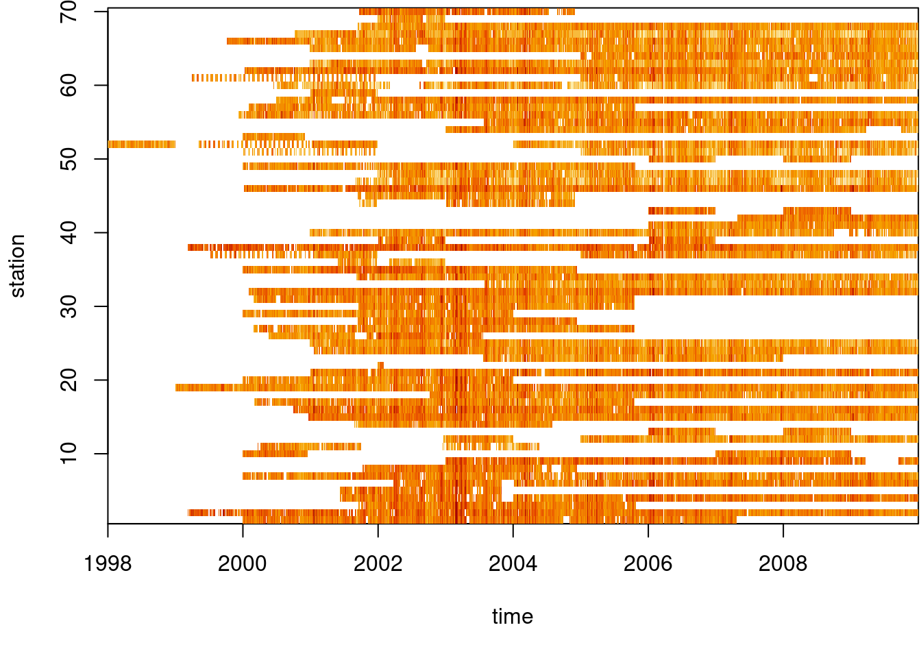
sparse space-time diagram of PM10 measurements by time and station

image code

par(mar = c(5.1, 4.1, 0.3, 0.1))
image(aperm(log(aq), 2:1), main = NULL)

image code

st_as_sf(st_apply(aq, 1, mean, na.rm = TRUE)) |>
    plot(reset = FALSE, pch = 16, extent = de_nuts1)
st_union(de_nuts1) |> plot(add = TRUE)

Example: aggregate these station time series to area means

(a <- aggregate(aq, de_nuts1, mean, na.rm = TRUE))

## stars object with 2 dimensions and 1 attribute
## attribute(s):
##         Min. 1st Qu.   Median     Mean  3rd Qu.     Max.  NA's
## PM10  1.0752 10.8855 15.31625 17.88823 21.81086 172.2665 25679
## dimension(s):
##      from   to     offset  delta refsys point
## geom    1   16         NA     NA WGS 84 FALSE
## time    1 4383 1998-01-01 1 days   Date FALSE
##                                                             values
## geom MULTIPOLYGON (((9.65046 4...,...,MULTIPOLYGON (((10.77189 ...
## time                                                          NULL

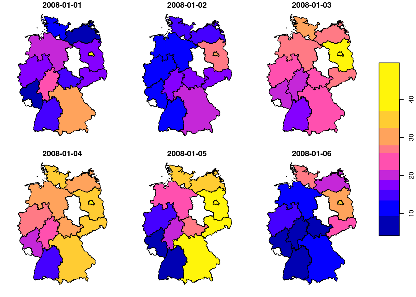
Example: show the maps for six arbitrarily chosen days

a |> filter(time >= "2008-01-01", time < "2008-01-07") |> 
    plot(key.pos = 4)

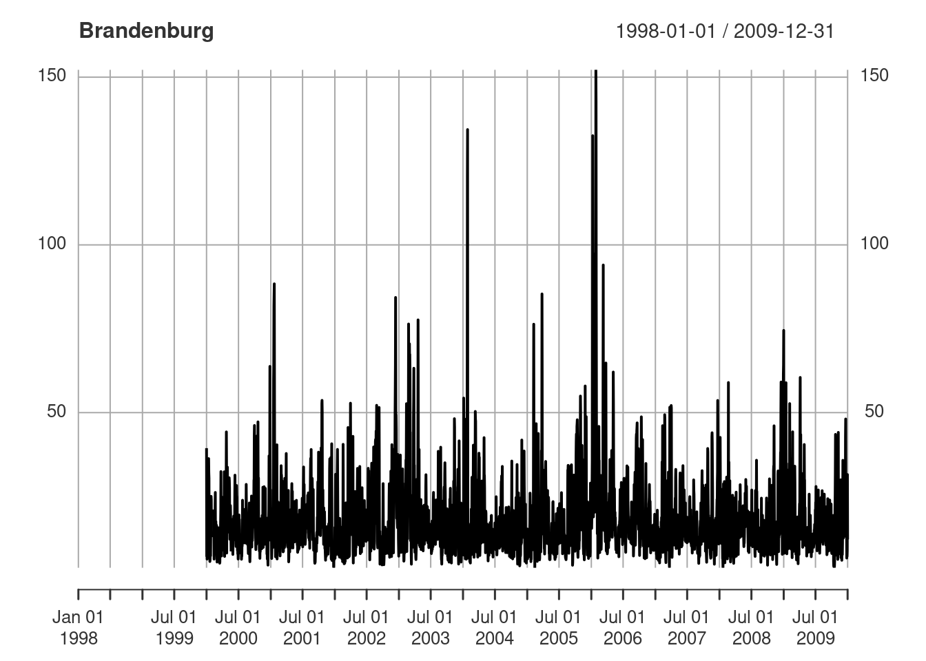
Example: time series plot of mean values for a single state

plot(as.xts(a)[,4], main = de_nuts1$NAME_1[4])