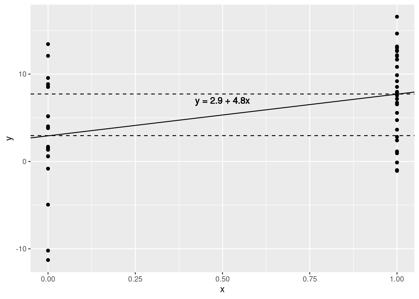
Estimating a difference = regressing on an indicator variable
Add a new group:
n_1 <- 30
y_1 <- rnorm(n_1, 8.0, 5.0)
diff <- mean(y_1) - mean(y_0)
se_0 <- sd(y_0)/sqrt(n_0)
se_1 <- sd(y_1)/sqrt(n_1)
se <- sqrt(se_0^2 + se_1^2)
cat(paste0("Diff: ",diff," Se: ", se))
## Diff: 4.76270151940131 Se: 1.72310260696003Compare to true difference of 6.0
As a regression (again with flat priors):
n <- n_0 + n_1
y <- c(y_0, y_1)
x <- c(rep(0, n_0), rep(1, n_1))
fake <- data.frame(x, y)
fit <- stan_glm(y ~ x, data=fake, prior_intercept=NULL, prior=NULL, prior_aux=NULL, refresh=0)
print(fit, detail=FALSE)
## Median MAD_SD
## (Intercept) 2.9 1.3
## x 4.8 1.7
##
## Auxiliary parameter(s):
## Median MAD_SD
## sigma 5.7 0.6Indicator slope (4.8) is the same as the difference in means
MAD_SD (1.5) is nearly the same as the the SE

Fake data simulation is a general tool that will continue to be helpful in more complicated settings.