13.7 Building a logisic regression model
- Instead of going through the well example, lets look at exercise 13.1. This uses the NES data but looking at more variables. There are 70 total in the data set. i picked out some of them. Note that there was also a ‘race’ categorical but I could not find figure out the categories. (A preliminary model not shown here indicates that race =2 is the only strong predictor)
part a+ b:
file_nes <- here::here("data/nes.txt")
nes92 <-
  file_nes %>%
  read.table() %>%
  as_tibble() %>%
  filter(year == 1992) %>%
  filter(xor(dvote, rvote)) %>%
  select(rvote, age, female, black, educ1, educ2, educ3, income)  %>%
  mutate(female = as.factor(female), black = as.factor(black))
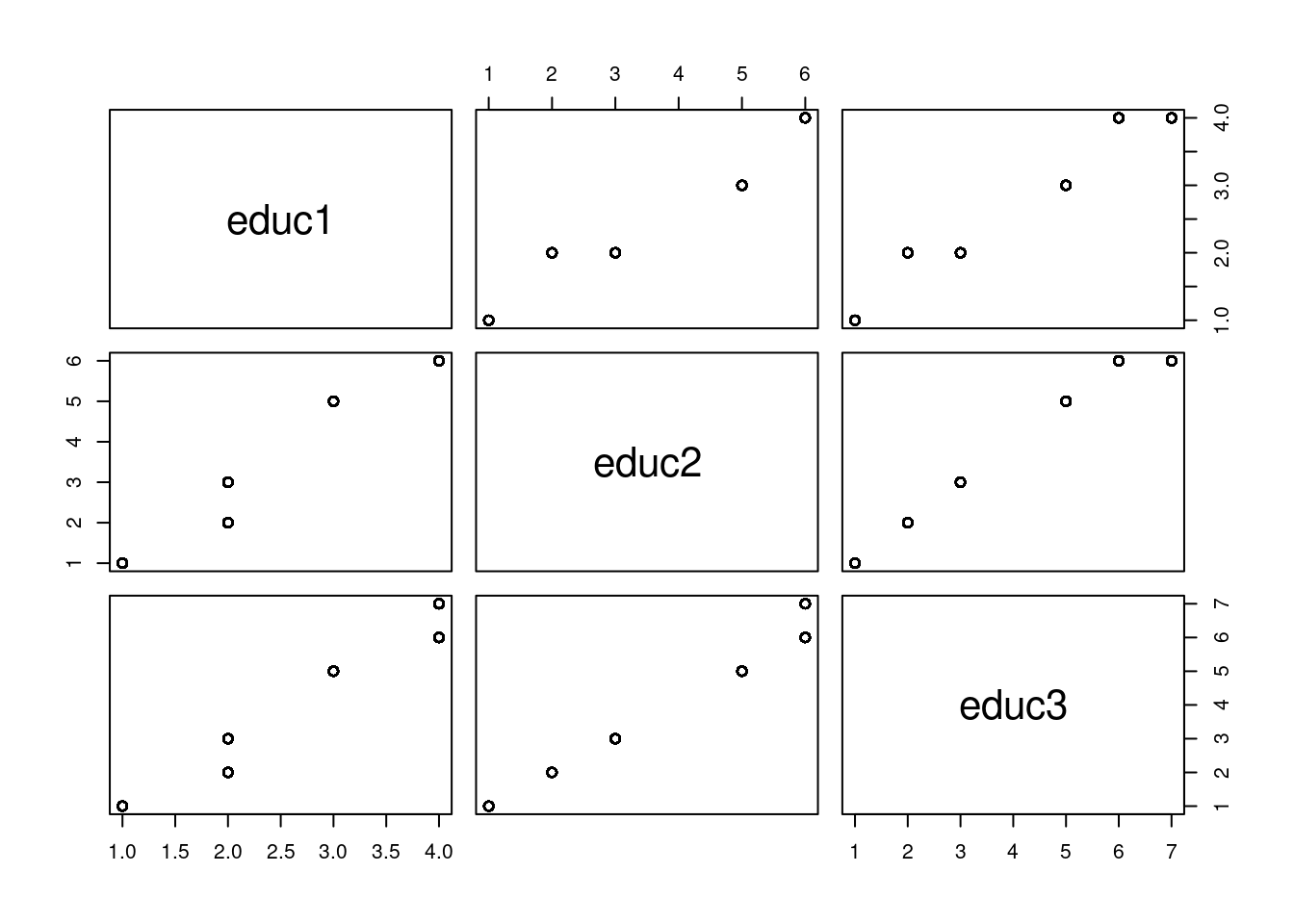
educ1 seems to be on a different scale. I am just going to combine 2 and 3 and call it good for this exercise.
I will treat education as continuous just as was done for income.
I included some interactions that apriori seem important
fit_all <- stan_glm(rvote ~ educ + black + income + female + age + age:black + income:black + female:income, data = nes92, family=binomial(link= 'logit'), refresh = 0)
print(fit_all, digits = 3)
## stan_glm
## family: binomial [logit]
## formula: rvote ~ educ + black + income + female + age + age:black + income:black +
## female:income
## observations: 1179
## predictors: 9
## ------
## Median MAD_SD
## (Intercept) -1.916 0.436
## educ 0.053 0.043
## black1 -4.024 1.652
## income 0.459 0.104
## female1 0.996 0.430
## age 0.002 0.004
## black1:age 0.028 0.021
## black1:income -0.055 0.333
## income:female1 -0.342 0.125
##
## ------
## * For help interpreting the printed output see ?print.stanreg
## * For info on the priors used see ?prior_summary.stanregLets look at loo. The baseline loo is
## [1] -817.047##
## Computed from 4000 by 1179 log-likelihood matrix.
##
## Estimate SE
## elpd_loo -727.9 12.0
## p_loo 8.5 0.9
## looic 1455.8 24.0
## ------
## MCSE of elpd_loo is 0.1.
## MCSE and ESS estimates assume MCMC draws (r_eff in [0.5, 1.3]).
##
## All Pareto k estimates are good (k < 0.7).
## See help('pareto-k-diagnostic') for details.Simplify a bit by droping the poorest predictors
fit_2 <- stan_glm(rvote ~ educ + black + income + age + female + female:income, data = nes92, family=binomial(link= 'logit'), refresh = 0)
print(fit_2, digits = 3)
## stan_glm
## family: binomial [logit]
## formula: rvote ~ educ + black + income + age + female + female:income
## observations: 1179
## predictors: 7
## ------
## Median MAD_SD
## (Intercept) -1.937 0.432
## educ 0.051 0.046
## black1 -2.745 0.377
## income 0.460 0.104
## age 0.003 0.004
## female1 0.999 0.423
## income:female1 -0.344 0.129
##
## ------
## * For help interpreting the printed output see ?print.stanreg
## * For info on the priors used see ?prior_summary.stanreg##
## Computed from 4000 by 1179 log-likelihood matrix.
##
## Estimate SE
## elpd_loo -727.2 11.8
## p_loo 7.1 0.4
## looic 1454.5 23.6
## ------
## MCSE of elpd_loo is 0.0.
## MCSE and ESS estimates assume MCMC draws (r_eff in [0.5, 1.2]).
##
## All Pareto k estimates are good (k < 0.7).
## See help('pareto-k-diagnostic') for details.Ok and lets try even simpler:
fit_3 <- stan_glm(rvote ~ black + income + female + female:income, data = nes92, family=binomial(link= 'logit'), refresh = 0)
print(fit_3, digits = 3)
## stan_glm
## family: binomial [logit]
## formula: rvote ~ black + income + female + female:income
## observations: 1179
## predictors: 5
## ------
## Median MAD_SD
## (Intercept) -1.678 0.345
## black1 -2.750 0.385
## income 0.488 0.098
## female1 1.009 0.418
## income:female1 -0.346 0.124
##
## ------
## * For help interpreting the printed output see ?print.stanreg
## * For info on the priors used see ?prior_summary.stanreg##
## Computed from 4000 by 1179 log-likelihood matrix.
##
## Estimate SE
## elpd_loo -726.1 11.7
## p_loo 5.1 0.4
## looic 1452.2 23.5
## ------
## MCSE of elpd_loo is 0.0.
## MCSE and ESS estimates assume MCMC draws (r_eff in [0.3, 1.0]).
##
## All Pareto k estimates are good (k < 0.7).
## See help('pareto-k-diagnostic') for details.Finally, leave out the last interaction:
fit_4 <- stan_glm(rvote ~ black + income + female, data = nes92, family=binomial(link= 'logit'), refresh = 0)
print(fit_4, digits = 3)
## stan_glm
## family: binomial [logit]
## formula: rvote ~ black + income + female
## observations: 1179
## predictors: 4
## ------
## Median MAD_SD
## (Intercept) -0.967 0.213
## black1 -2.718 0.377
## income 0.272 0.060
## female1 -0.103 0.125
##
## ------
## * For help interpreting the printed output see ?print.stanreg
## * For info on the priors used see ?prior_summary.stanreg## elpd_diff se_diff
## fit_3 0.0 0.0
## fit_2 -1.2 1.3
## fit_all -1.8 1.9
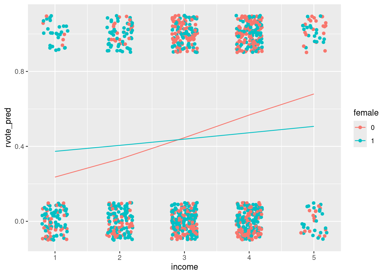
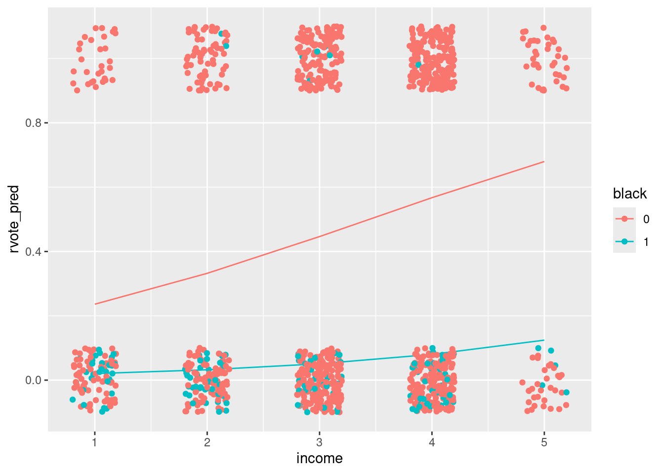
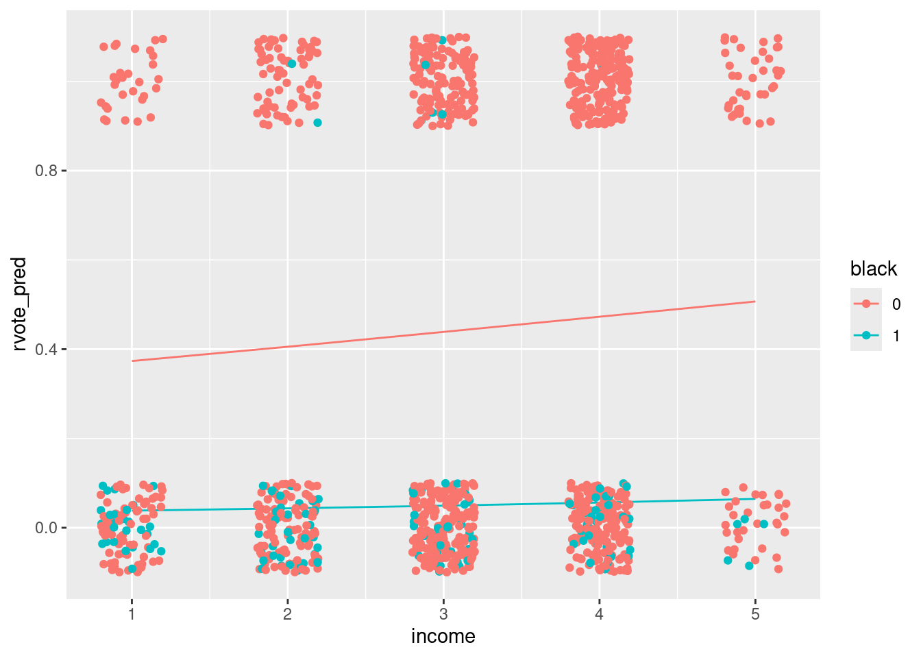
## fit_4 -3.0 2.8From this, the simplest fit with the interaction is best, but it is not strongly significant.
- Looking at fit_3, what are the important variables? Discuss during meeting.
QUESTION: How can I set up this test data tibble in a less labor intensive way?
test_data = tibble(income = rep(seq(1:5),4), female =c(rep(1,10), rep(0,10)), black = rep(c(rep(0,5), rep(1,5)),2))
test_data$female = as.factor(test_data$female)
test_data$black = as.factor(test_data$black)test_data$rvote_pred = predict(fit_3, newdata = test_data, type="response")
test_data %>% filter(black == 0) %>%
ggplot()+ geom_line(aes(x=income, y=rvote_pred, color = female)) +
geom_jitter(aes(x=income, y=rvote, color=female), width = .2, height = .1, data=nes92)
test_data %>% filter(female == 0) %>%
ggplot()+ geom_line(aes(x=income, y=rvote_pred, color = black)) +
     geom_jitter(aes(x=income, y=rvote, color=black), width = .2, height = .1, data=nes92)
test_data %>% filter(female == 1) %>%
ggplot()+ geom_line(aes(x=income, y=rvote_pred, color = black)) +
     geom_jitter(aes(x=income, y=rvote, color=black), width = .2, height = .1, data=nes92)