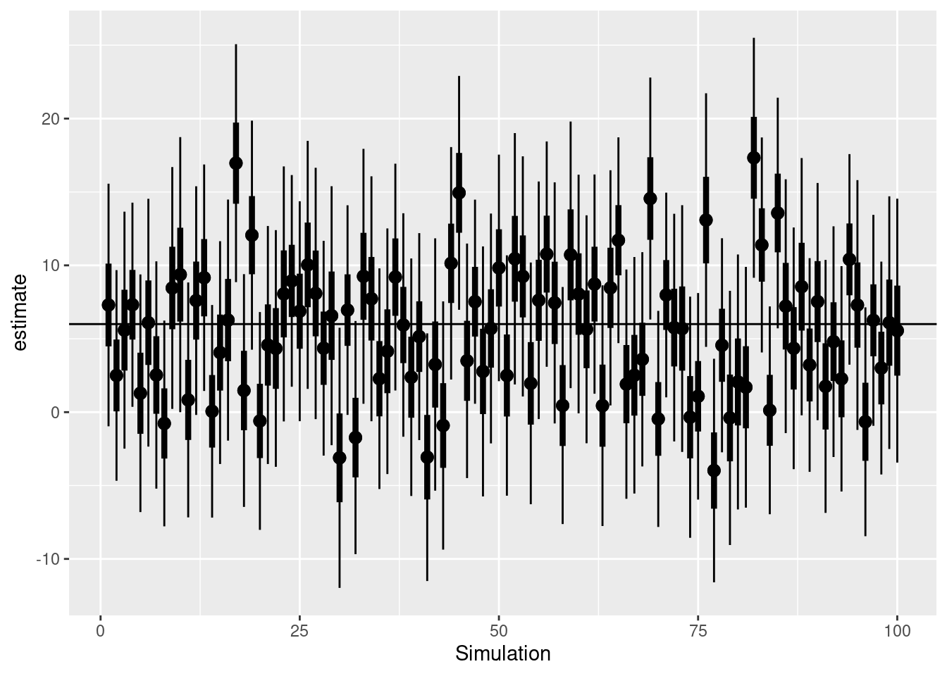
Confidence Interval Simulation

This is simulation of 100 draws from a distribution with mean 6 and standard deviation 40. The standard error will be close to 4.

library(dplyr)
library(ggplot2)
set.seed(42)
mu <- 6
sig <- 40
n_draws <- 100
n_reps <- 1000

sim_coverage <- tibble(
  estimate = rep(0,n_reps), se = estimate
)


for(i in 1:n_reps){
 sim_data <- rnorm(n_draws,mean=mu, sd= sig)
 sim_coverage$estimate[[i]] <- mean(sim_data)
 sim_coverage$se[[i]] = sd(sim_data)/sqrt(n_draws)
}

sim_coverage <- sim_coverage |>
 mutate(min_95 = qt(0.025,n_draws-1)*se + estimate,
        max_95 = qt(0.975,n_draws-1)*se + estimate,
        min_50 = qt(0.25,n_draws-1)*se + estimate,
        max_50 = qt(0.75,n_draws-1)*se + estimate,
        covered_95 = min_95 <= mu & max_95 >= mu,
        covered_50 = min_50 <= mu & max_50 >= mu
        )
ggplot(head(sim_coverage,100),aes(x= 1:100, y = estimate)) +
  geom_pointrange(aes(ymin = min_95,ymax = max_95))+
  geom_pointrange(aes(ymin = min_50,ymax = max_50), linewidth= 1.5) +
  geom_hline(aes(yintercept=6)) +
  xlab('Simulation')

We expect on about 50% of the time that the 50% CI contains the true value, while we expect 95% of the time that the 95% CI contains the true value.

sim_coverage |> summarise(p_covered_95 = mean(sim_coverage$covered_95),
                          p_covered_50 = mean(sim_coverage$covered_50))       

## # A tibble: 1 × 2
##   p_covered_95 p_covered_50
##          <dbl>        <dbl>
## 1        0.953        0.493