Compare simulated with observed

Recall from previous chapter, we can more simply simulate using posterior_predict().

set.seed(970)
y_rep <- posterior_predict(fit)
# Each row of the matrix y_rep is 66 columns of simulated `newcomb` data

Verify these are the same thing (using same seed).

v <- matrix(y_rep_tidy$y, nrow = n_sims, ncol = n_newcomb, byrow = TRUE)

max(abs(y_rep - v))

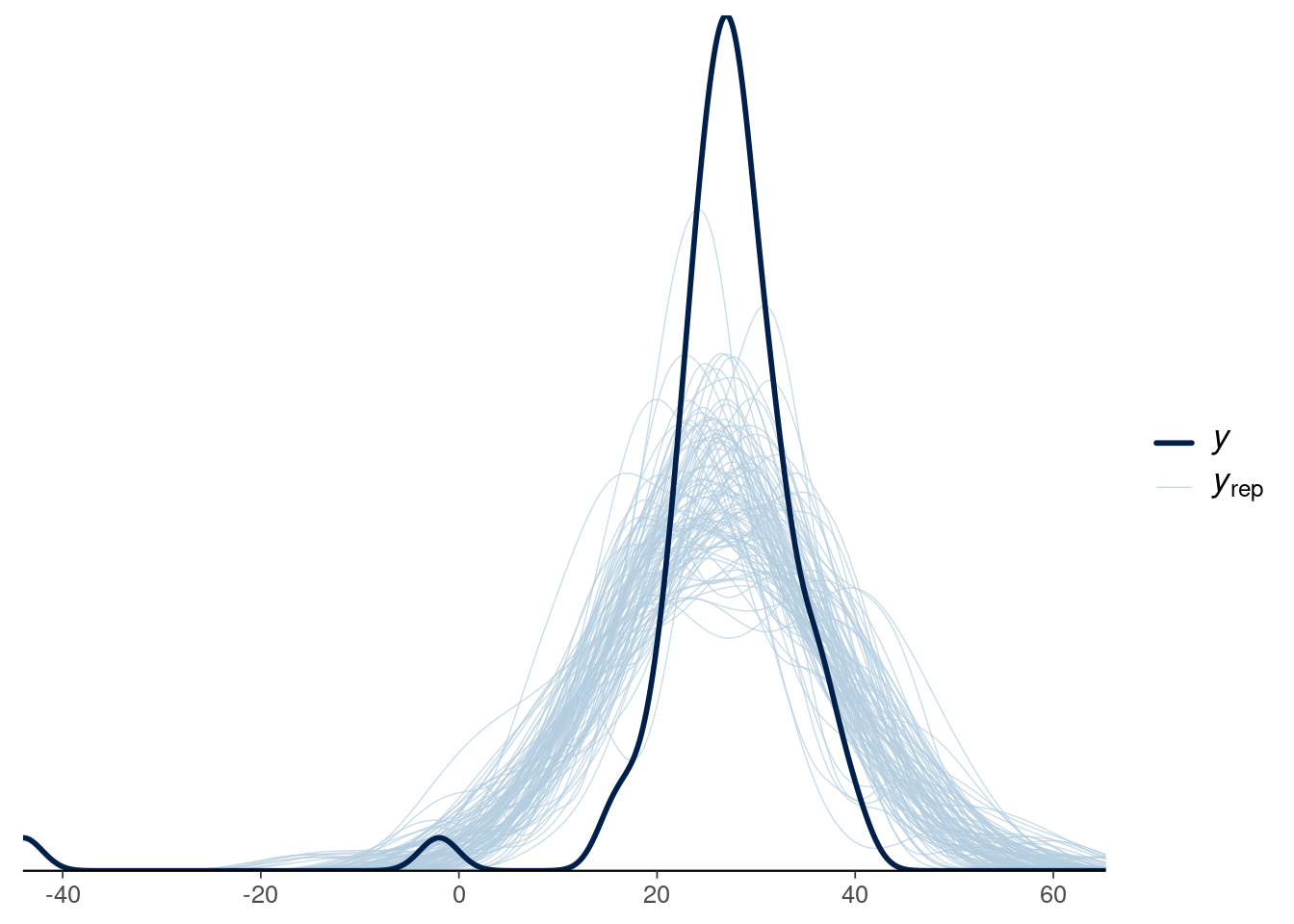
## [1] 0

We can use bayesplot package to plot kernel density of data and n_rep sample replicates t.

set.seed(792)

n_rep <- 100

sims_sample <- sample(n_sims, n_rep)

ppc_dens_overlay(y = newcomb$y, yrep = y_rep[sims_sample, ]) +
  theme(
    axis.line.y = element_blank(),
    text = element_text(family = "sans")
  )

Checking model fit using a numerical data summary

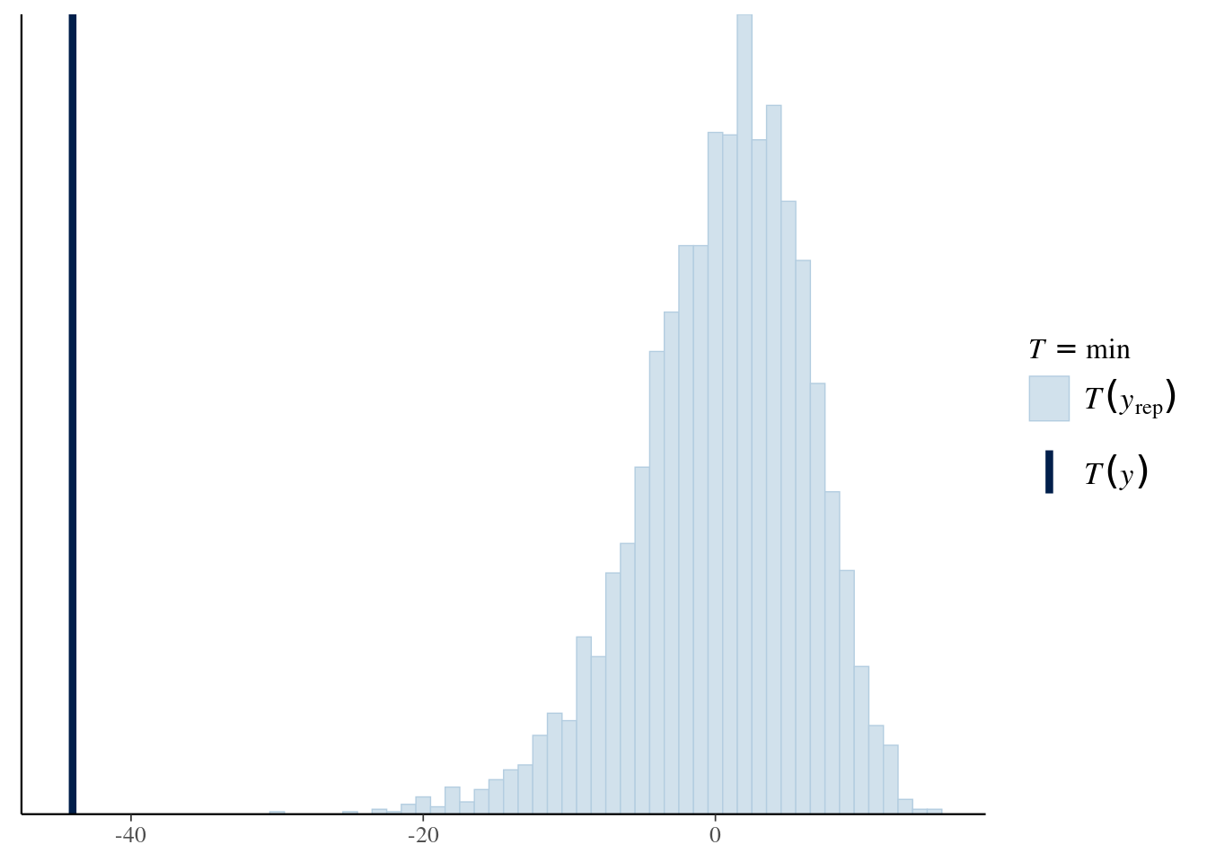
Choose your own statistic! Here we choose the minimum measurement.

Plot test statistic for data and replicates using bayesplot.

ppc_stat(y = newcomb$y, yrep = y_rep, stat = min, binwidth = 1)

A normal model clearly doesn’t work, a revised model might use an asymmetric distribution or long tailed distribution in place of the normal.