4.5 Regression Diagnostics

4.5.1 Outliers (extreme value) This may not be an influential case

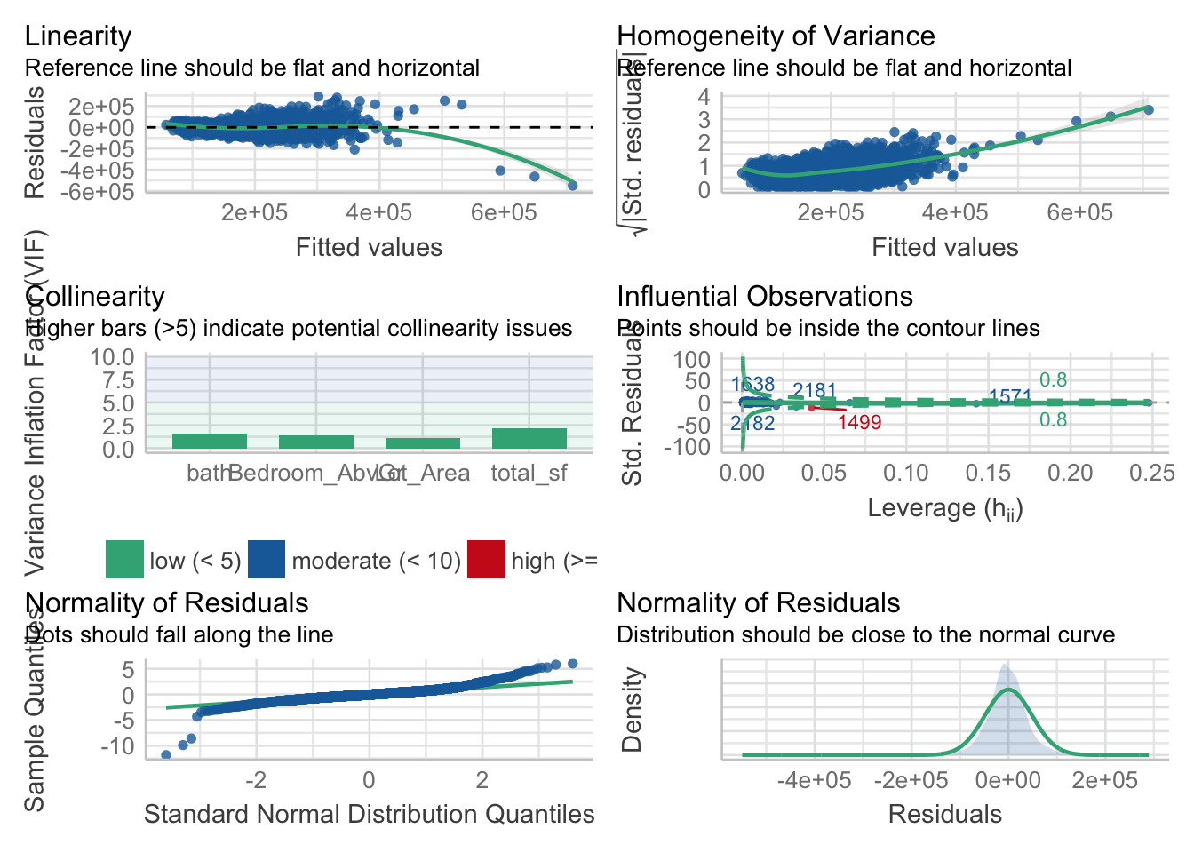
Using the {performance} package by Daniel Lüdecke, we identify one influential case using Cook’s Distance (Other options are available).

model <- lm(Sale_Price ~ total_sf+ bath + Lot_Area + Bedroom_AbvGr, data = dat)

outliers <- performance::check_outliers(model)
plot(outliers)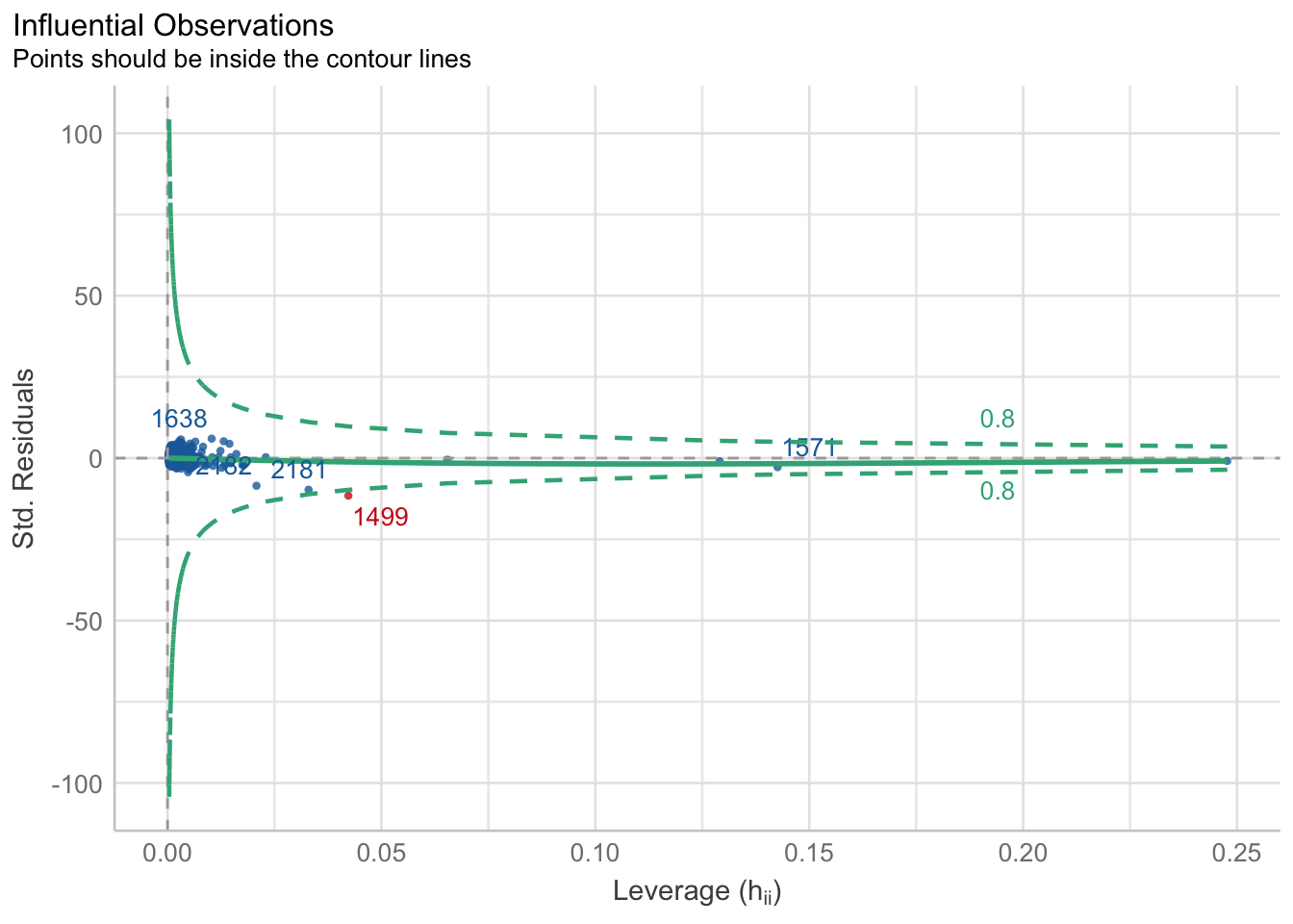

as.data.frame(outliers) %>% 
  dplyr::arrange(-Outlier_Cook) %>% 
  head()

##    Obs Distance_Cook Outlier_Cook Outlier
## 1 1499  1.178359e+00            1       1
## 2    1  5.037865e-05            0       0
## 3    2  2.824976e-07            0       0
## 4    3  6.201489e-05            0       0
## 5    4  1.308948e-04            0       0
## 6    5  4.909392e-06            0       0

It is hard to tell whether this is a typo or a one off sale. The property sold for $160k but has an almost 64k lot area and over 5.6k square footage–quite a deal in this area.

dat %>% slice(1499) %>% select(Sale_Price, total_sf, bath, Lot_Area, Bedroom_AbvGr)

## # A tibble: 1 × 5
##   Sale_Price total_sf  bath Lot_Area Bedroom_AbvGr
##        <int>    <int> <dbl>    <int>         <int>
## 1     160000     5642   4.5    63887             3

When we remove this influential case, our coefficients change quite a bit.

house_noinfluence <- lm(Sale_Price ~ total_sf+ bath + Lot_Area + Bedroom_AbvGr, 
                        data = dat %>% 
                          slice(1:1498, 1500:n()))

round(cbind(house_lm = model$coefficients,
                house_noinfluence = house_noinfluence$coefficients), digits = 3)

##                 house_lm house_noinfluence
## (Intercept)    28569.669         26596.755
## total_sf         104.848           109.716
## bath           28167.404         27124.051
## Lot_Area           0.622             0.742
## Bedroom_AbvGr -25683.007        -27089.435

4.5.2 Assumption Checking (Heteroscedasticity, Normality of residuals, Linearity, and Collinearity)

performance::check_model(model)