Histograms & Friends
state <- read.csv("data/state.csv")
head(state)
##        State Population Murder.Rate Abbreviation
## 1    Alabama    4779736         5.7           AL
## 2     Alaska     710231         5.6           AK
## 3    Arizona    6392017         4.7           AZ
## 4   Arkansas    2915918         5.6           AR
## 5 California   37253956         4.4           CA
## 6   Colorado    5029196         2.8           CO
library(ggplot2)
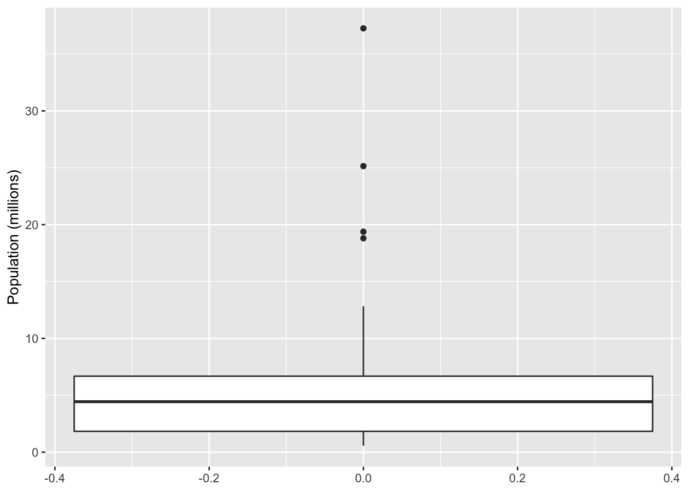
ggplot(state, aes(y = Population/1000000)) +
geom_boxplot() +
ylab("Population (millions)")
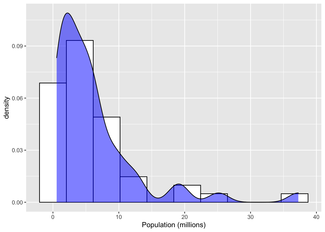
ggplot(state, aes(x = Population/1000000)) +
  geom_histogram(
    aes(y = after_stat(density)),
    bins = 10, fill = "white", color = "black"
  ) +
  geom_density(fill = "blue", alpha = 0.5) +
  xlab("Population (millions)")