4.6 Non-linear Regression

4.6.1 Partial Residual Plots and Nonlinearity

The linearity plot gives us some indication of a non-linear fit. To dig deeper, we can look at partial residual plots using the {ggeffects} package by Daniel Lüdecke. A partial residual plot represents the residuals of one dependent and one independent variable taking into account the other independent variables.

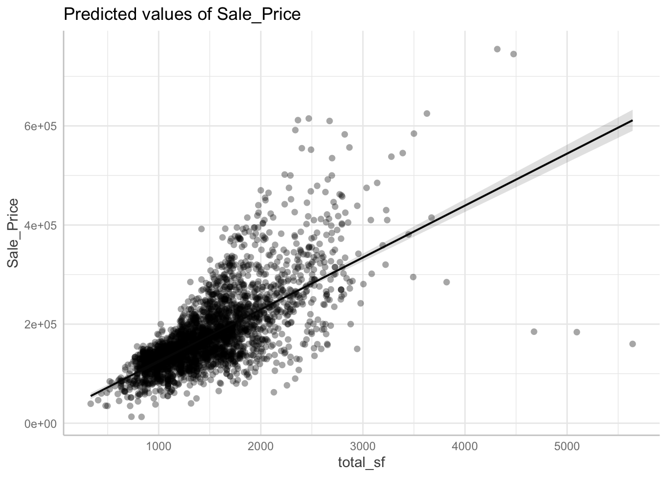
Here is a standard scatterplot between Sales Price and Total Square Feet

pr <- ggeffects::ggpredict(model, "total_sf [all]")
plot(pr, add.data = TRUE)

Here we produce a partial residual plot between Sales Price and Total Square Feet (taking into account the other independent variables). The blue line is a local polynomial regression line (loess) for reference. This indicates we may have a non-linear association.

plot(pr, residuals = TRUE, residuals.line = TRUE)

## `geom_smooth()` using formula 'y ~ x'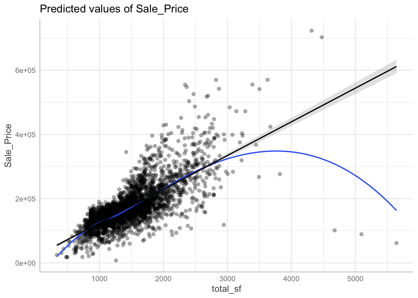

4.6.2 Polynomial and Spline Regression

We can create a polynomial variable (predictor squared) and add it into the model. The polynomial model seems to more accurately represent these data.

poly_model <- lm(Sale_Price ~ poly(total_sf, 2) + bath + Lot_Area + Bedroom_AbvGr, 
                 data = dat)

polynomial <- ggeffects::ggpredict(poly_model, "total_sf")
plot(polynomial, residuals = TRUE, residuals.line = TRUE)

## `geom_smooth()` using formula 'y ~ x'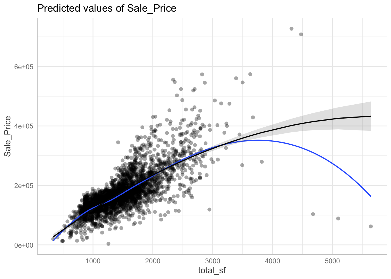

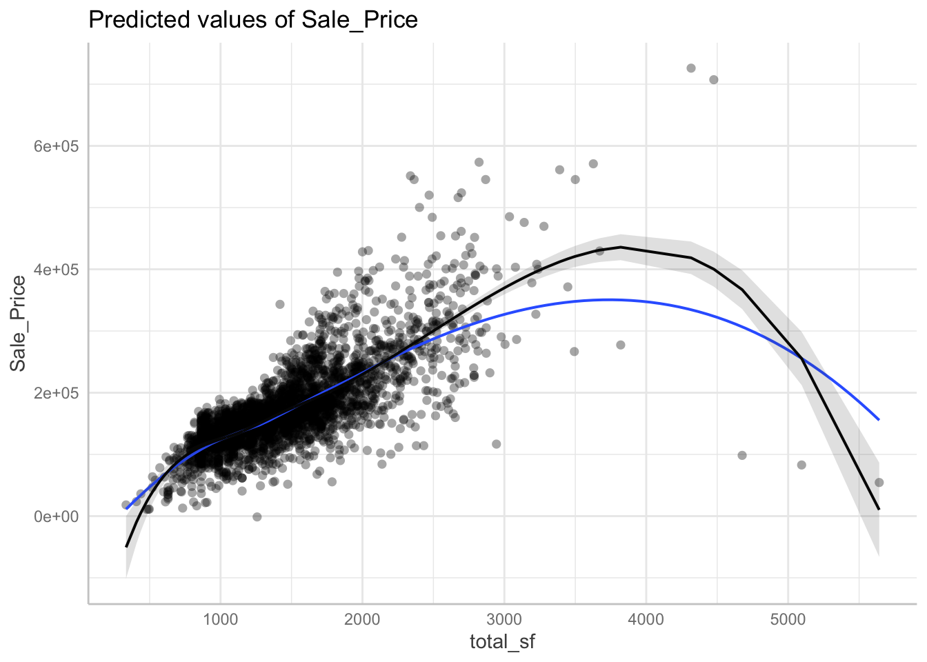
We can create a spline regression which will divides the dataset into multiple bins, called knots, and creates a separate fit for each bin. The difficult part is determining the correct knots.

knots <- quantile(dat$total_sf, p = c(0.25, 0.5, 0.75))
lm_spline <- lm(Sale_Price ~ splines::bs(total_sf, knots = knots, degree = 3) + 
                  bath + Lot_Area + Bedroom_AbvGr, data = dat)
spline <- ggeffects::ggpredict(lm_spline, "total_sf")
plot(spline, residuals = TRUE, residuals.line = TRUE)

## `geom_smooth()` using formula 'y ~ x'