5.2 Spatial neighborhood matrices
Packages needed:
library(tidyverse)
library(sf)
library(spdep)
library(SpatialEpi)
library(INLA)
library(cowplot)
A spatial model is a particular type of model as it takes consideration of autocorrelation between spatial points and so some weights are considered to identify the points’ proximity.
\[y=\sum_{i=1}^n{w_if(x_i)}\]
\(\mathit{W}\) is the proximity matrix or the inverse distance between areas and spatially connects areas \(i\) and \(j\), its elements \((i,j)\) , are:
\[i=(1,...,n)\] \[j=(1,...,m)\]
\[W=\begin{bmatrix} (1,1) & (1,2) & ... & (1,j)\\ (2,1) & ... & ... & (2,j)\\ ... & ... & ... & ...\\ (i,1) & ...& ... &(i,j)\\ \end{bmatrix}\]
The most simple cases are:
\[w_{i,j}=\left\{\begin{matrix} 1 & \text{ if i and j share same boundaries}\\ 0 & \text{ otherwise} \end{matrix}\right.\]
As an alternative, a standardized matrix can be used, adjusted for the total number of neighbors in each area:
\[w_{std,i,j}=\frac{w_{i,j}}{\sum_{j=1}^n{w_{ij}}}\]
Let’s have a look at the data: Lung Cancer in Pennsylvania
# install.packages("SpatialEpi")
# library(SpatialEpi)

map <- pennLC$spatial.polygon
plot(map)
And construct the neighbors list for each county:
# install.packages("spdep")
# library(spdep)
nb <- spdep::poly2nb(map)
nb%>%class
[1] "nb"head(nb,3)[[1]]
[1] 21 28 67
[[2]]
[1] 3 4 10 63 65
[[3]]
[1] 2 10 16 32 33 65d <- data.frame(county = names(map),
neigh = rep(0, length(map)))
rownames(d) <- names(map)
map <- SpatialPolygonsDataFrame(map, d, match.ID = TRUE)
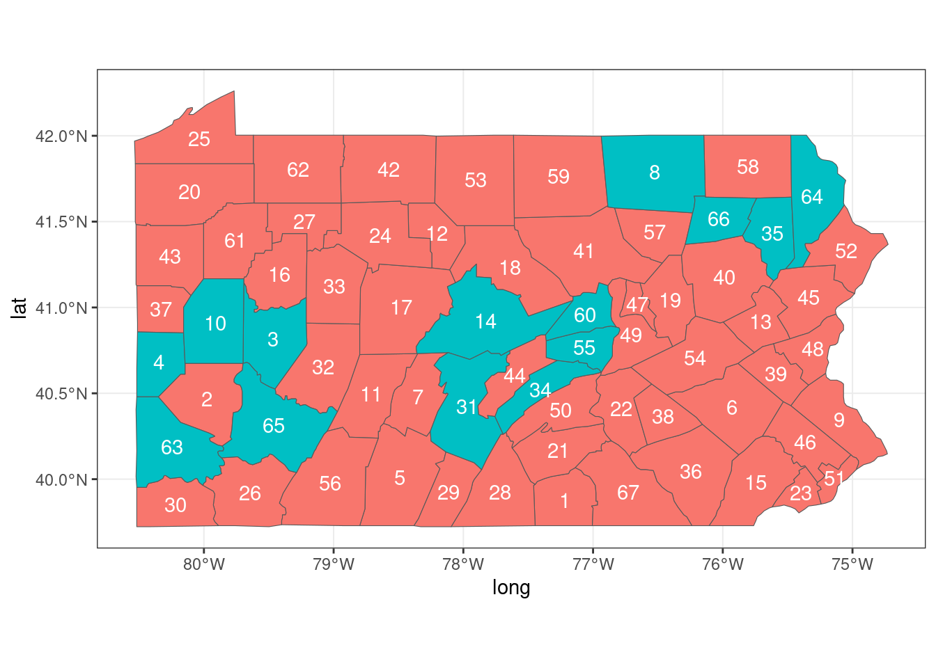
map$neigh[nb[[2]]] <- 1
map$neigh[nb[[44]]] <- 1
map$neigh[nb[[58]]] <- 1
map%>%as_tibble()%>%head# A tibble: 6 × 2
county neigh
<chr> <dbl>
1 adams 0
2 allegheny 0
3 armstrong 1
4 beaver 1
5 bedford 0
6 berks 0coord <- coordinates(map)
map$long <- coord[, 1]
map$lat <- coord[, 2]
map$ID <- 1:dim(map@data)[1]
map@proj4string## Coordinate Reference System:
## Deprecated Proj.4 representation: +proj=longlatmap%>%as_tibble()%>%head## # A tibble: 6 × 5
## county neigh long lat ID
## <chr> <dbl> <dbl> <dbl> <int>
## 1 adams 0 -77.2 39.9 1
## 2 allegheny 0 -80.0 40.5 2
## 3 armstrong 1 -79.5 40.8 3
## 4 beaver 1 -80.3 40.7 4
## 5 bedford 0 -78.5 40.0 5
## 6 berks 0 -75.9 40.4 6# install.packages("sf")
# library(sf)
mapsf <- sf::st_as_sf(map)# ggplot(mapsf)+
# geom_sf()
ggplot(mapsf) +
geom_sf(aes(fill = as.factor(neigh))) +
geom_text(aes(long, lat, label = ID), color = "white") +
guides(fill = "none") +
theme_bw() 
Figure 5.1: Neighbors of areas 2, 44 and 58 of Pennsylvania