11.6 Figures
Figures can be created by writing the R code that generates them inside an R code chunk. In the R chunk we can write the option fig.cap to write a caption, and fig.align to specify the alignment of the figure (‘left’, ‘center’ or ‘right’). We can also use out.width and out.height to specify the size of the output. For example, out.width = ‘80%’ means the output occupies 80% of the page width.
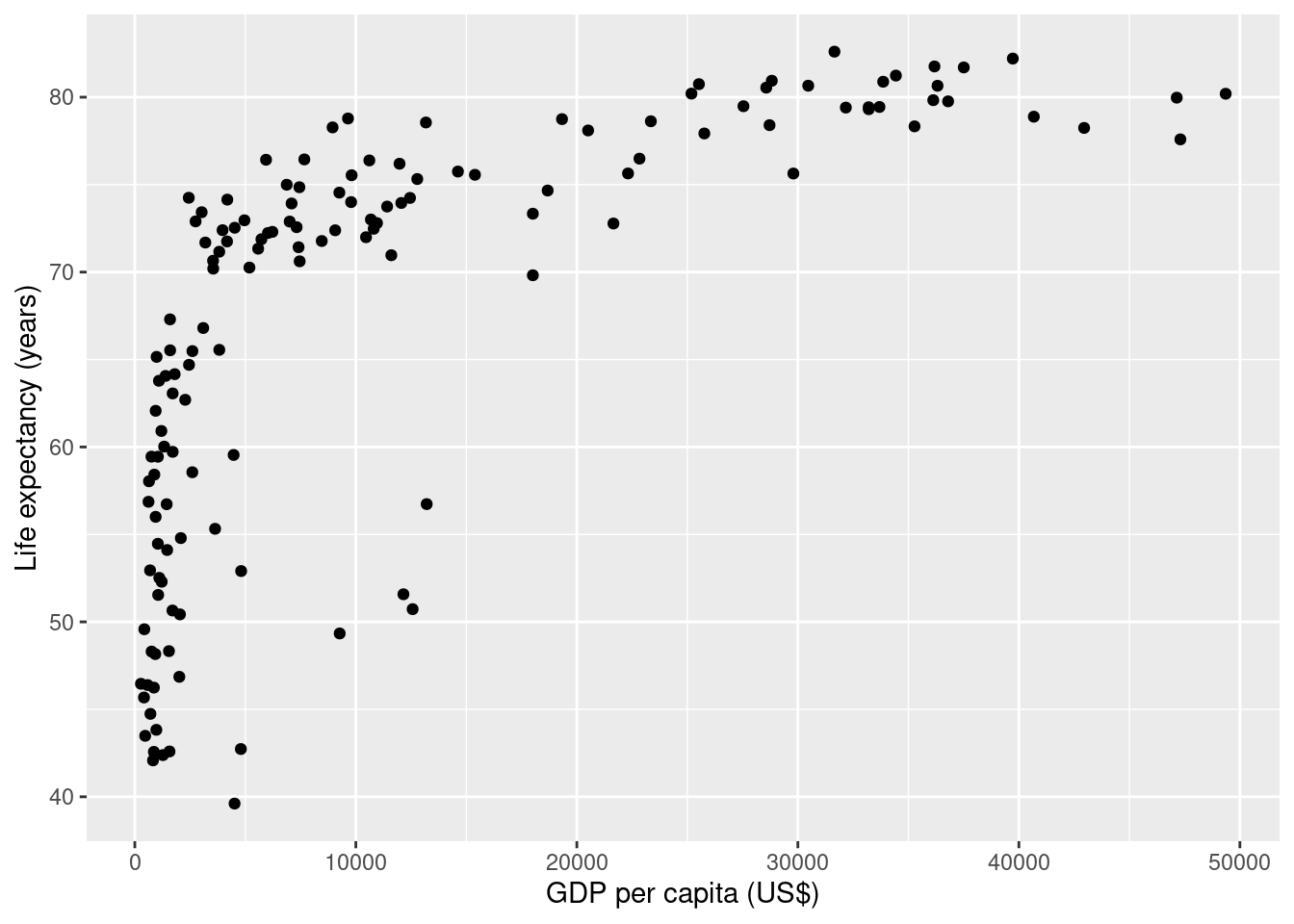
The following chunk creates a scatterplot with life expectancy at birth versus GDP per capita in 2007 obtained from the gapminder data. The chunk uses fig.cap to specify a caption for the figure.
library(ggplot2)
ggplot(
  gapminder[which(gapminder$year == 2007), ],
  aes(x = gdpPercap, y = lifeExp)
) +
geom_point() +
  xlab("GDP per capita (US$)") +
  ylab("Life expectancy (years)")
Figure 11.1: Life expectancy versus GDP per capita in 2007.
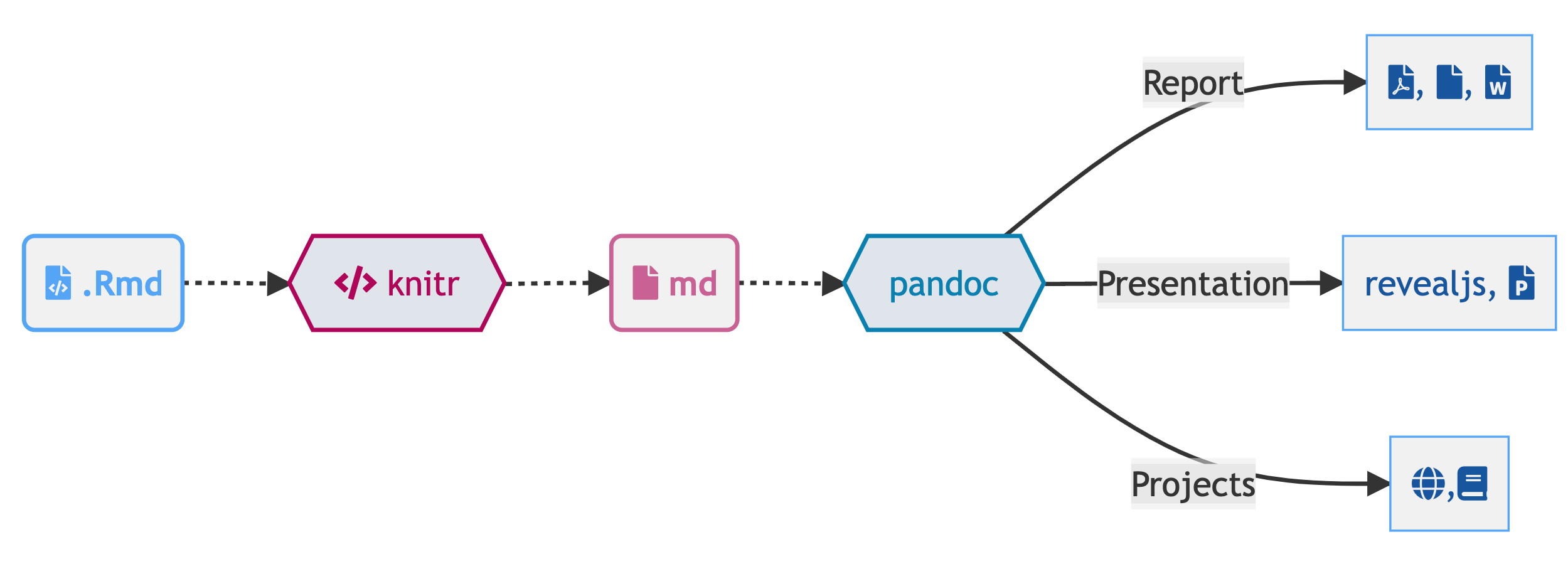
Images that are already saved can also be easily included with Markdown syntax. For example, if the image is saved in path path/img.png, it can be included in the document using

rmarkdown workflow
We can also include the image with the include_graphics() function of the knitr package. This allows to specify chunk options. For example, we can include a centered figure that occupies 25% of the document and has caption.
knitr::include_graphics("path/img.png")