17.6 How it’s used when taking time series seriously

• some events impact all groups
  1. summarize groups into one (but losing information)
  2. treat each group separately, and use separate regressions
  3. aggregate with regression, $\beta_i$ being a group FE

$$Outcome = \beta_i + \beta_1t + \beta_2 After + \beta_3 t \times After + \epsilon$$

• event matters differently over time
  • leave out time just before the event kicks in
  • standard errors for each period
  • everything is relative to the period before the event

$$Outcome = \beta_0 + \beta_t + \epsilon$$

library(tidyverse); library(fixest)
set.seed(10)

# Create data with 10 groups and 10 time periods
df <- crossing(id = 1:10, t = 1:10) %>%
 # Add an event in period 6 with a one-period positive effect
 mutate(Y = rnorm(n()) + 1*(t == 6))

# Use i() in feols to include time dummies,
# specifying that we want to drop t = 5 as the reference
m <- feols(Y ~ i(t, ref = 5), data = df,
 cluster = 'id')

# Plot the results, except for the intercep,# and add a line joining 
# them and a space and line for the reference group
coefplot(m, drop = '(Intercept)',
 pt.join = TRUE, ref = c('t:5' = 6), ref.line = TRUE)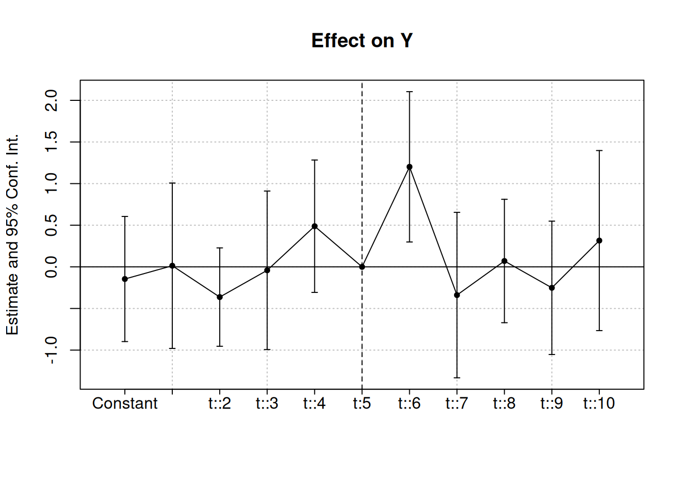

• significant where we expect it ($t = 6$)
• unexpectedly significant ($t = 2$ and $t = 4$) b/c small sample