17.4 How it’s used in Finance

• stock prices reflect information about a company
• short time window

1. estimation period before event, observation period from just before the event to the period of interest after event
2. use estimation period data to predict $\hat{R}$ (predicted stock returns)
   • means-adjusted returns model
   • market-adjusted returns model
   • risk-adjusted returns model
3. In observation period: $AR = R - \hat{R}$ to get abnormal return
4. consider AR in observation period

Example

• estimation period: May–July
• observation period: August 6 – August 24

library(tidyverse); library(lubridate)

## ── Attaching core tidyverse packages ──────────────────────── tidyverse 2.0.0 ──
## ✔ dplyr     1.1.4     ✔ readr     2.1.5
## ✔ forcats   1.0.0     ✔ stringr   1.5.1
## ✔ ggplot2   3.5.1     ✔ tibble    3.2.1
## ✔ lubridate 1.9.4     ✔ tidyr     1.3.1
## ✔ purrr     1.0.4     
## ── Conflicts ────────────────────────────────────────── tidyverse_conflicts() ──
## ✖ dplyr::filter() masks stats::filter()
## ✖ dplyr::lag()    masks stats::lag()
## ℹ Use the conflicted package (<http://conflicted.r-lib.org/>) to force all conflicts to become errors

goog <- causaldata::google_stock

event <- ymd("2015-08-10")

# Create estimation data set
est_data <- goog %>%
 filter(Date >= ymd('2015-05-01') &
 Date <= ymd('2015-07-31'))

# And observation data
obs_data <- goog %>%
 filter(Date >= event - days(4) & 
 Date <= event + days(14))

# Estimate a model predicting stock price with market return
m <- lm(Google_Return ~ SP500_Return, data = est_data)

# Get AR
obs_data <- obs_data %>%
 # Using mean of estimation return
 mutate(AR_mean = Google_Return - mean(est_data$Google_Return),
 # Then comparing to market return
 AR_market = Google_Return - SP500_Return,
 # Then using model fit with estimation data
 risk_predict = predict(m, newdata = obs_data),
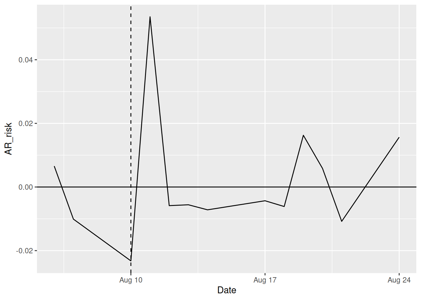
 AR_risk = Google_Return - risk_predict)

# Graph the results
ggplot(obs_data, aes(x = Date, y = AR_risk)) + 
 geom_line() + 
 geom_vline(aes(xintercept = event), linetype = 'dashed') + 
 geom_hline(aes(yintercept = 0))