13.4 Tools for efficient grid search

A few tricks:

13.4.1 Submodel optimization

Types of models where, from a single model fit, multiple tuning parameters can be evaluated without refitting:

• Partial Least Squares (no. of components to retain)

• Boosting models (no. of boosting iterations, i.e. trees)

• glmnet makes (across the amount of regularization)

• MARS adds a set of nonlinear features (number of terms to retain)

The tune package automatically applies this type of optimization whenever an applicable model is tuned. See also this vignette

methods("multi_predict")

##  [1] multi_predict._C5.0*        multi_predict._earth*      
##  [3] multi_predict._elnet*       multi_predict._glmnetfit*  
##  [5] multi_predict._lognet*      multi_predict._multnet*    
##  [7] multi_predict._torch_mlp*   multi_predict._train.kknn* 
##  [9] multi_predict._xgb.Booster* multi_predict.default*     
## see '?methods' for accessing help and source code

parsnip:::multi_predict._C5.0 %>% 
  formals() %>% 
  names()

## [1] "object"   "new_data" "type"     "trees"    "..."

For example, if a C5.0 model is fit to this cell classification data challenge, we can tune the trees. With all other parameters set at their default values, we can rapidly evaluate iterations from 1 to 100 :

data(cells)

cells <- cells %>% select(-case)

cell_folds <- vfold_cv(cells)

roc_res <- metric_set(roc_auc)

c5_spec <- 
  boost_tree(trees = tune()) %>% 
  set_engine("C5.0") %>% 
  set_mode("classification")

set.seed(2)
c5_tune <- c5_spec %>%
  tune_grid(
    class ~ .,
    resamples = cell_folds,
    grid = data.frame(trees = 1:100),
    metrics = roc_res
  )

Even though we fit the model without the submodel prediction trick, this optimization is automatically applied by parsnip.

autoplot(c5_tune)

ggsave("images/13_c5_submodel.png")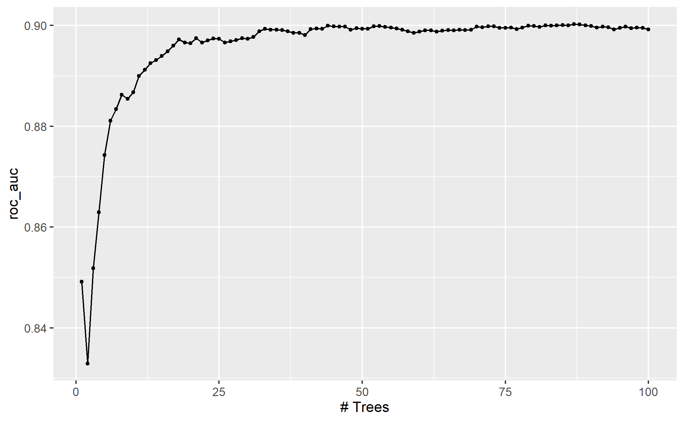

13.4.2 Parallel processing

backend packages right now are doFuture, doMC, doMPI, doParallel, doRedis,doRNG, doSNOW, and doAzureParallel

In tune_*(), there are two approaches, often set in control_grid() or control_resamples()

• parallel_over = "resamples or

• parallel_over = "everything" or

• parallel_over = NULL (the default) chooses “resamples” if there are more than one resample, otherwise chooses “everything” to attempt to maximize core utilization

Note that switching between parallel_over strategies is not guaranteed to use the same random number generation schemes. However, re-tuning a model using the same parallel_over strategy is guaranteed to be reproducible between runs.

To use them, register the parallel backend first.

On a shared server, never never consume all of the cores.

all_cores <- parallel::detectCores(logical = FALSE)

library(doParallel)
cl <- makePSOCKcluster(all_cores)
doParallel::registerDoParallel(cl)

Be careful to avoid use of variables from the global environment. For example:

num_pcs <- 3

recipe(mpg ~ ., data = mtcars) %>% 
  # Bad since num_pcs might not be found by a worker process
  step_pca(all_predictors(), num_comp = num_pcs)

recipe(mpg ~ ., data = mtcars) %>% 
  # Good since the value is injected into the object
  step_pca(all_predictors(), num_comp = !!num_pcs)

for the most part, the logging provided by tune_grid() will not be seen when running in parallel.

13.4.3 Benchmarking Parallel with boosted trees

Three scenarios

1. Preprocess the data prior to modeling using dplyr

2. Conduct the same preprocessing via a recipe

3. With a recipe, add a step that has a high computational cost

using variable numbers of worker processes and using the two parallel_over options, on a computer with 10 physical cores

For dplyr and the simple recipe

• There is little difference in the execution times between the panels.

• There is some benefit for using parallel_over = "everything" with many cores. However, as shown in the figure, the majority of the benefit of parallel processing occurs in the first five workers.

With the expensive preprocessing step, there is a considerable difference in execution times. Using parallel_over = "everything" is problematic since, even using all cores, it never achieves the execution time that parallel_over = "resamples" attains with just five cores. This is because the costly preprocessing step is unnecessarily repeated in the computational scheme.

Overall, note that the increased computational savings will vary from model-to-model and are also affected by the size of the grid, the number of resamples, etc. A very computationally efficient model may not benefit as much from parallel processing.

13.4.4 Racing Methods

The finetune package contains functions for racing.

One issue with grid search is that all models need to be fit across all resamples before any tuning parameters can be evaluated. It would be helpful if instead, at some point during tuning, an interim analysis could be conducted to eliminate any truly awful parameter candidates.

In racing methods the tuning process evaluates all models on an initial subset of resamples. Based on their current performance metrics, some parameter sets are not considered in subsequent resamples.

As an example, in the Chicago multilayer perceptron tuning process with a regular grid above, what would the results look like after only the first three folds?

We can fit a model where the outcome is the resampled area under the ROC curve and the predictor is an indicator for the parameter combination. The model takes the resample-to-resample effect into account and produces point and interval estimates for each parameter setting. The results of the model are one-sided 95% confidence intervals that measure the loss of the ROC value relative to the currently best performing parameters.

Any parameter set whose confidence interval includes zero would lack evidence that its performance is not statistically different from the best results. We retain 10 settings; these are resampled more. The remaining 10 submodels are no longer considered.

Racing methods can be more efficient than basic grid search as long as the interim analysis is fast and some parameter settings have poor performance. It also is most helpful when the model does not have the ability to exploit submodel predictions.

The tune_race_anova() function conducts an Analysis of Variance (ANOVA) model to test for statistical significance of the different model configurations.

library(finetune)

set.seed(99)
mlp_sfd_race <-
  mlp_wflow %>%
  tune_race_anova(
    Chicago_folds,
    grid = 20,
    param_info = mlp_param,
    metrics = rmse_mape_rsq_iic,
    control = control_race(verbose_elim = TRUE)
  )

write_rds(mlp_sfd_race, 
          "data/13-Chicago-mlp_sfd_race.rds",
          compress = "gz")

autoplot(mlp_sfd_race)

ggsave("images/13_mlp_sfd_race.png",
       width = 12)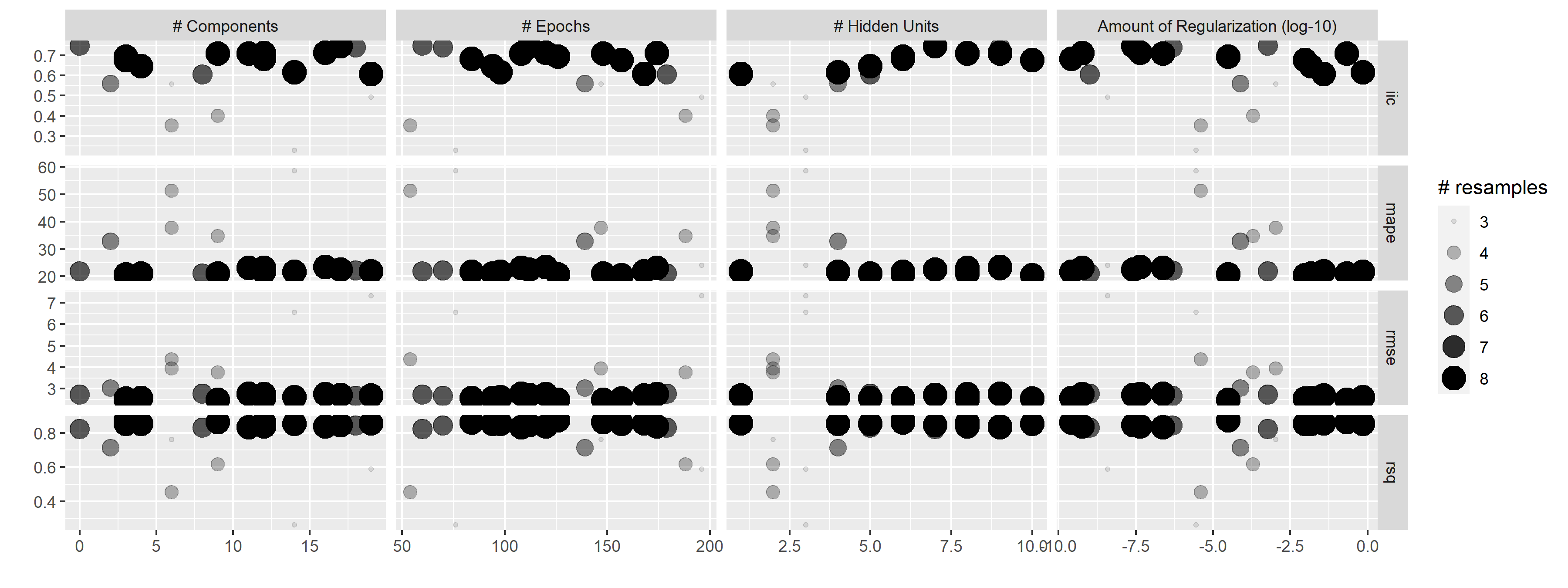

show_best(mlp_sfd_race, n = 6)

  hidden_units  penalty epochs num_comp .metric .estimator  mean     n
         <int>    <dbl>  <int>    <int> <chr>   <chr>      <dbl> <int>
1            6 3.08e- 5    126        3 rmse    standard    2.47     8
2            8 2.15e- 1    148        9 rmse    standard    2.48     8
3           10 9.52e- 3    157        3 rmse    standard    2.55     8
4            6 2.60e-10     84       12 rmse    standard    2.56     8
5            5 1.48e- 2     94        4 rmse    standard    2.57     8
6            4 7.08e- 1     98       14 rmse    standard    2.60     8
# ... with 2 more variables: std_err <dbl>, .config <chr>
Warning message:
No value of `metric` was given; metric 'rmse' will be used.