15.1 Obligatory Setup

Using the 2021 World Happiness Report. Why?

• Small
• Interesting

How I felt reading this chapter with concrete from {modeldata}

library(tidyverse)
library(tidymodels)
theme_set(theme_minimal(base_size = 16))

df <- 
  here::here('data', 'world-happiness-report-2021.csv') %>%
  read_csv() %>% 
  janitor::clean_names()

df %>% skimr::skim()

Tabla 15.1: Data summary

Name	Piped data
Number of rows	149
Number of columns	20
_______________________
Column type frequency:
character	2
numeric	18
________________________
Group variables	None

Variable type: character

skim_variable	n_missing	complete_rate	min	max	empty	n_unique	whitespace
country_name	0	1	4	25	0	149	0
regional_indicator	0	1	9	34	0	10	0

Variable type: numeric

skim_variable	n_missing	complete_rate	mean	sd	p0	p25	p50	p75	p100	hist
ladder_score	0	1	5.53	1.07	2.52	4.85	5.53	6.26	7.84	▁▅▇▇▃
standard_error_of_ladder_score	0	1	0.06	0.02	0.03	0.04	0.05	0.07	0.17	▇▆▁▁▁
upperwhisker	0	1	5.65	1.05	2.60	4.99	5.62	6.34	7.90	▁▃▇▇▃
lowerwhisker	0	1	5.42	1.09	2.45	4.71	5.41	6.13	7.78	▁▃▇▇▃
logged_gdp_per_capita	0	1	9.43	1.16	6.64	8.54	9.57	10.42	11.65	▂▆▇▇▅
social_support	0	1	0.81	0.11	0.46	0.75	0.83	0.90	0.98	▁▂▃▇▇
healthy_life_expectancy	0	1	64.99	6.76	48.48	59.80	66.60	69.60	76.95	▂▃▃▇▅
freedom_to_make_life_choices	0	1	0.79	0.11	0.38	0.72	0.80	0.88	0.97	▁▂▅▇▇
generosity	0	1	-0.02	0.15	-0.29	-0.13	-0.04	0.08	0.54	▅▇▅▁▁
perceptions_of_corruption	0	1	0.73	0.18	0.08	0.67	0.78	0.84	0.94	▁▁▁▅▇
ladder_score_in_dystopia	0	1	2.43	0.00	2.43	2.43	2.43	2.43	2.43	▁▁▇▁▁
explained_by_log_gdp_per_capita	0	1	0.98	0.40	0.00	0.67	1.02	1.32	1.75	▂▆▇▇▅
explained_by_social_support	0	1	0.79	0.26	0.00	0.65	0.83	1.00	1.17	▁▂▅▇▇
explained_by_healthy_life_expectancy	0	1	0.52	0.21	0.00	0.36	0.57	0.66	0.90	▂▃▃▇▅
explained_by_freedom_to_make_life_choices	0	1	0.50	0.14	0.00	0.41	0.51	0.60	0.72	▁▂▅▇▇
explained_by_generosity	0	1	0.18	0.10	0.00	0.10	0.16	0.24	0.54	▅▇▅▁▁
explained_by_perceptions_of_corruption	0	1	0.14	0.11	0.00	0.06	0.10	0.17	0.55	▇▅▁▁▁
dystopia_residual	0	1	2.43	0.54	0.65	2.14	2.51	2.79	3.48	▁▂▅▇▃

library(corrr)
df_selected <-
  df %>%
  select(
    ladder_score,
    logged_gdp_per_capita,
    social_support,
    healthy_life_expectancy,
    freedom_to_make_life_choices,
    generosity,
    perceptions_of_corruption
  )

cors <-
  df_selected %>% 
  select(where(is.numeric)) %>% 
  corrr::correlate() %>% 
  rename(col1 = term) %>% 
  pivot_longer(
    -col1,
    names_to = 'col2',
    values_to = 'cor'
  ) %>% 
  arrange(desc(abs(cor)))
cors %>% filter(col1 == 'ladder_score')

## # A tibble: 7 × 3
##   col1         col2                             cor
##   <chr>        <chr>                          <dbl>
## 1 ladder_score logged_gdp_per_capita         0.790 
## 2 ladder_score healthy_life_expectancy       0.768 
## 3 ladder_score social_support                0.757 
## 4 ladder_score freedom_to_make_life_choices  0.608 
## 5 ladder_score perceptions_of_corruption    -0.421 
## 6 ladder_score generosity                   -0.0178
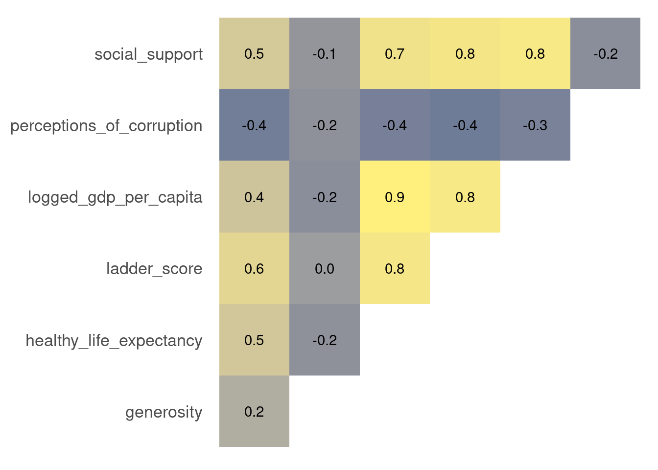
## 7 ladder_score ladder_score                 NA

p_cors <-
  cors %>% 
  filter(col1 < col2) %>% 
  ggplot() +
  aes(x = col1, y = col2) +
  geom_tile(aes(fill = cor), alpha = 0.7) +
  geom_text(aes(label = scales::number(cor, accuracy = 0.1))) +
  guides(fill = "none") +
  scale_fill_viridis_c(option = 'E', direction = 1, begin = 0.2) +
  labs(x = NULL, y = NULL) +
  theme(
    panel.grid.major = element_blank(),
    axis.text.x = element_blank()
  )
p_cors