9.3 Regression Metrics
Load in the Data
library(tidymodels)
library(glmnet)
library(ranger)
set.seed(1123)
data(ames)

ames <- ames %>%
  mutate(
    under_budget = as.factor(if_else(Sale_Price<=160000,1,0)),
    Sale_Price = log10(Sale_Price))
#Cross-fold validation
ames_folds <- vfold_cv(ames, v = 5)
#Create Recipe
ames_recipe <-
recipe(formula = Sale_Price ~ Gr_Liv_Area + Full_Bath + Half_Bath + Lot_Area + Neighborhood + Overall_Cond,
data = ames) %>%
step_dummy(all_nominal())
#Set the model and hyperparameters
ames_spec <-
linear_reg(penalty = tune(), mixture = tune()) %>%
set_mode("regression") %>%
set_engine("glmnet")
#Create workflow
ames_workflow <-
workflow() %>%
add_recipe(ames_recipe) %>%
add_model(ames_spec)
#Create metric set of all regression metrics
ames_tune <-
tune_grid(
ames_workflow,
metrics =
metric_set(rmse, rsq, rsq_trad, mae, mpe, mape, smape, mase, ccc, rpiq, rpd, huber_loss, huber_loss_pseudo, iic),
resamples = ames_folds,
grid = grid_latin_hypercube(penalty(), mixture(), size = 8)
)
#Pick the best model for each metric and pull out the predictions
best_models <-
tibble(
metric_name = c('rmse', 'rsq', 'rsq_trad', 'mae', 'mpe', 'mape', 'smape', 'mase',
'ccc','rpiq', 'rpd', 'huber_loss', 'huber_loss_pseudo', 'iic')) %>%
mutate(metric_best = map(metric_name, ~select_best(ames_tune, .x)),
wf_best = map(metric_best, ~finalize_workflow(ames_workflow, .x)),
fit_best = map(wf_best, ~fit(.x, data = ames)),
df_pred = map(fit_best, ~ames %>% bind_cols(predict(.x, new_data = ames)) %>% select(Sale_Price, .pred))) %>%
select(-c(wf_best, fit_best)) %>%
unnest(cols = c(metric_name, metric_best, df_pred))
#Plot!
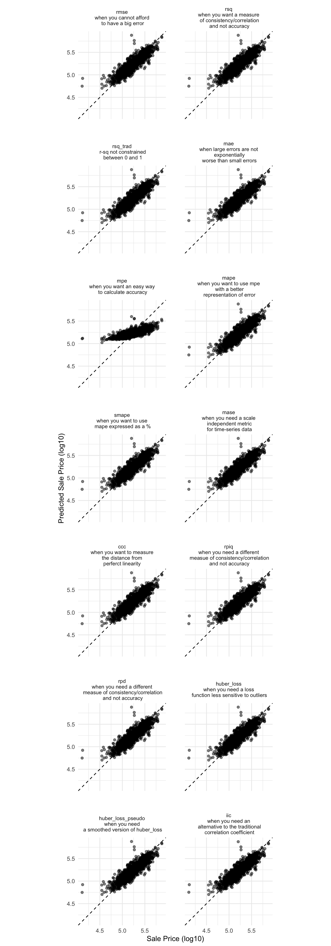
best_models %>%
mutate(metric_desc = factor(
metric_name,
levels = c('rmse', 'rsq', 'rsq_trad', 'mae', 'mpe', 'mape', 'smape', 'mase',
'ccc','rpiq', 'rpd', 'huber_loss', 'huber_loss_pseudo', 'iic'),
labels = c('rmse\nwhen you cannot afford\n to have a big error',
'rsq\nwhen you want a measure\n of consistency/correlation\n and not accuracy',
'rsq_trad\n r-sq not constrained\n between 0 and 1',
'mae\nwhen large errors are not\n exponentially\n worse than small errors',
'mpe\nwhen you want an easy way\n to calculate accuracy',
'mape\nwhen you want to use mpe\n with a better\n representation of error',
'smape\nwhen you want to use\n mape expressed as a %',
'mase\nwhen you need a scale\n independent metric\n for time-series data',
'ccc\nwhen you want to measure\n the distance from \nperferct linearity',
'rpiq\nwhen you need a different\n measue of consistency/correlation\n and not accuracy',
'rpd\nwhen you need a different\n measue of consistency/correlation\n and not accuracy',
'huber_loss\nwhen you need a loss\n function less sensitive to outliers',
'huber_loss_pseudo\nwhen you need\n a smoothed version of huber_loss',
'iic\nwhen you need an\n alternative to the traditional\n correlation coefficient'))) %>%
ggplot(aes(x = Sale_Price, y = .pred)) +
geom_abline(lty = 2) +
geom_point(alpha = 0.5) +
labs(y = "Predicted Sale Price (log10)", x = "Sale Price (log10)") +
coord_obs_pred() +
facet_wrap(~metric_desc, ncol = 2) +
theme_minimal() +
theme(panel.spacing = unit(2, "lines"),
strip.text.x = element_text(size = 8))
best_models %>% select(metric_name, penalty, mixture) %>% distinct()## # A tibble: 14 × 3
## metric_name penalty mixture
## <chr> <dbl> <dbl>
## 1 rmse 1.74e- 6 0.887
## 2 rsq 6.71e-10 0.112
## 3 rsq_trad 1.74e- 6 0.887
## 4 mae 1.74e- 6 0.887
## 5 mpe 1.66e- 1 0.163
## 6 mape 1.74e- 6 0.887
## 7 smape 1.74e- 6 0.887
## 8 mase 1.74e- 6 0.887
## 9 ccc 6.71e-10 0.112
## 10 rpiq 6.71e-10 0.112
## 11 rpd 6.71e-10 0.112
## 12 huber_loss 1.74e- 6 0.887
## 13 huber_loss_pseudo 1.74e- 6 0.887
## 14 iic 3.81e- 4 0.552