11.5 Random graphs galore
One problem is that we are basing our analysis on a single random graph. Because edges are drawn randomly, there is a lot of variation in the structure of random graphs, especially when the number of nodes in the graph is small (less than one thousand).
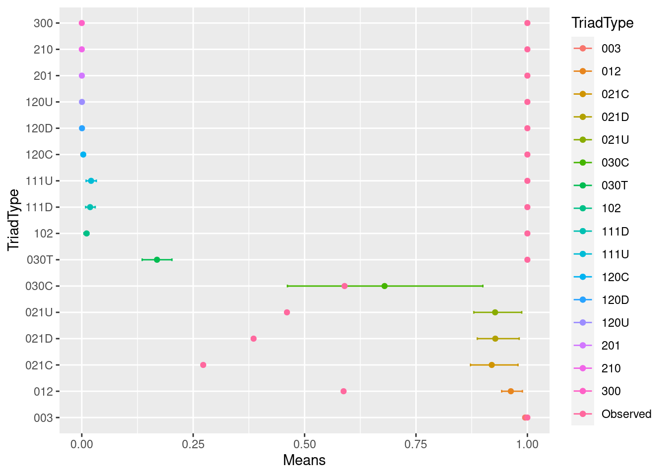
What we really want is a distribution of random graphs and their triad censuses, against which our own could be compared. So let’s generate one hundred random graphs, and create a distribution of random graph triad censuses and see where our graph lies on that distribution
trial <- vector("list", 100) # this creates a list with 100 spaces to store things.  We will store each result here.

trial <- lapply(seq(100), function(x){
  random_graph <- erdos.renyi.game(n = net59_n, p.or.m = net59_density, directed = TRUE)
  triad.census(random_graph)
})


trial_df <- do.call("rbind", trial) # We can use the do.call and "rbind" functions together to combine all of the results into a matrix, where each row is one of our trials

colnames(trial_df) <- c("003", "012", "102", "021D", "021U", "021C", "111D", "111U", "030T", "030C", "201", "120D", "120U", "120C", "210", "300") # It is worth naming the columns too.

trial_df_w_observed <- rbind(trial_df, as.numeric(triad.census(net59))) # add in the observed results
# First, standardize all of the columns by dividing each of their values by the largest value in that column, so that each will be on a similar scale (0 to 1), we can visualize them meaningfully
trial_df_w_observed <- as.data.frame(trial_df_w_observed)
trial_df_w_observed[,1:ncol(trial_df_w_observed)] <- sapply(trial_df_w_observed[,1:length(trial_df_w_observed)], function(x) x/max(x))
# Then split the observed from the simulation results
trial_df <- as.data.frame(trial_df_w_observed[1:100,])
observed <- as.numeric(trial_df_w_observed[101,])
# Summarize the simulation results and add the observed data set back in for comparison
summarized_stats <- data.frame(TriadType = colnames(trial_df),
Means = sapply(trial_df, mean),
LowerCI = sapply(trial_df, function(x) quantile(x, 0.05)),
UpperCI = sapply(trial_df, function(x) quantile(x, 0.95)),
Observed = observed)
summarized_stats## TriadType Means LowerCI UpperCI Observed
## 003 003 0.9948345802 0.994071010 0.9954347900 1.0000000
## 012 012 0.9628859418 0.942326115 0.9887844619 0.5875339
## 102 102 0.0108590651 0.004875651 0.0158361233 1.0000000
## 021D 021D 0.9279801959 0.887611797 0.9815694208 0.3855409
## 021U 021U 0.9275492388 0.879782817 0.9872671138 0.4604493
## 021C 021C 0.9200247969 0.872451725 0.9788962752 0.2725018
## 111D 111D 0.0187313803 0.008676763 0.0300769613 1.0000000
## 111U 111U 0.0208897485 0.009671180 0.0326333241 1.0000000
## 030T 030T 0.1688000000 0.135555556 0.2023333333 1.0000000
## 030C 030C 0.6794871795 0.461538462 0.9000000000 0.5897436
## 201 201 0.0001570167 0.000000000 0.0009813543 1.0000000
## 120D 120D 0.0004761905 0.000000000 0.0034013605 1.0000000
## 120U 120U 0.0004062500 0.000000000 0.0031250000 1.0000000
## 120C 120C 0.0032846715 0.000000000 0.0076642336 1.0000000
## 210 210 0.0000000000 0.000000000 0.0000000000 1.0000000
## 300 300 0.0000000000 0.000000000 0.0000000000 1.0000000ggplot(summarized_stats) +
geom_point(aes(x=TriadType, y=Means, colour=TriadType)) +
geom_errorbar(aes(x = TriadType, ymin=LowerCI, ymax=UpperCI, colour=TriadType), width=.1) +
geom_point(aes(x=TriadType, y=Observed, colour="Observed")) +
coord_flip()