14.3 Performing Kriging in R

To perform Kriging in R, you can use the gstat package, which provides functions for geostatistical analysis. The gstat package allows you to create a variogram model, fit the model to the data, and use the model to interpolate values at unobserved locations.

library(gstat)

14.3.1 Example: Simple Kriging

In this example, we will perform simple Kriging on a dataset of air quality measurements. We will estimate the air quality at unobserved locations based on the measurements at nearby monitoring stations.

Step 1: Load the air quality data and create a variogram model.

library(sp)
# Load the air quality data
data(meuse)
coordinates(meuse) <- c("x", "y")
meuse%>%
  as_data_frame()%>%
  select(x,y,zinc)%>%
  head()

## # A tibble: 6 × 3
##        x      y  zinc
##    <dbl>  <dbl> <dbl>
## 1 181072 333611  1022
## 2 181025 333558  1141
## 3 181165 333537   640
## 4 181298 333484   257
## 5 181307 333330   269
## 6 181390 333260   281

Step 2: Visualize the data.

meuse%>%
  as_data_frame()%>%
  select(x,y,zinc)%>%
  ggplot(aes(x,y,color=zinc))+
  geom_point()+
  scale_color_viridis_c()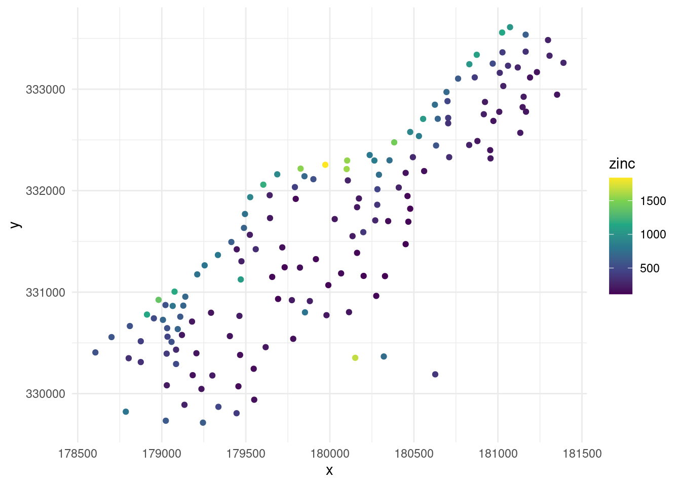

What we need is a grid of points where we want to predict the zinc concentration.

data(meuse.grid)
meuse.grid %>%
  as_data_frame()%>%
  select(x,y)%>%
  ggplot(aes(x,y))+
  geom_point(shape=".")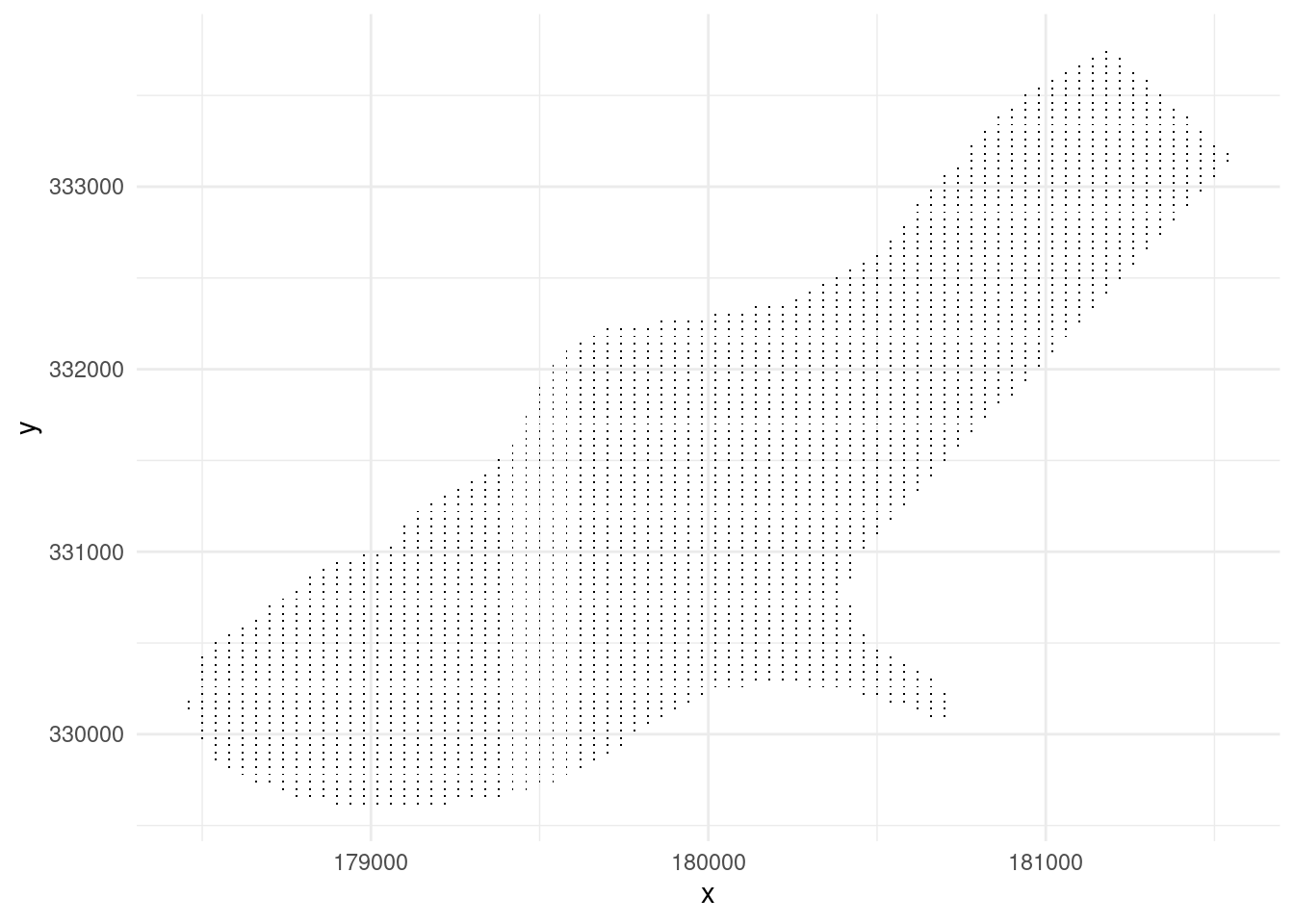

zinc_data <- meuse%>%
  as_data_frame()%>%
  select(x,y,zinc)

grid_data <- meuse.grid %>%
  as_data_frame()%>%
  select(x,y)

ggplot()+
  geom_point(data=grid_data,aes(x,y),shape=".")+
  geom_point(data=zinc_data,aes(x,y,color=zinc))+
  scale_color_viridis_c()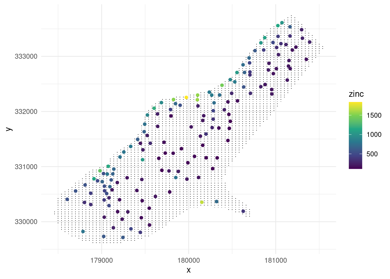

14.3.2 Variogram Model

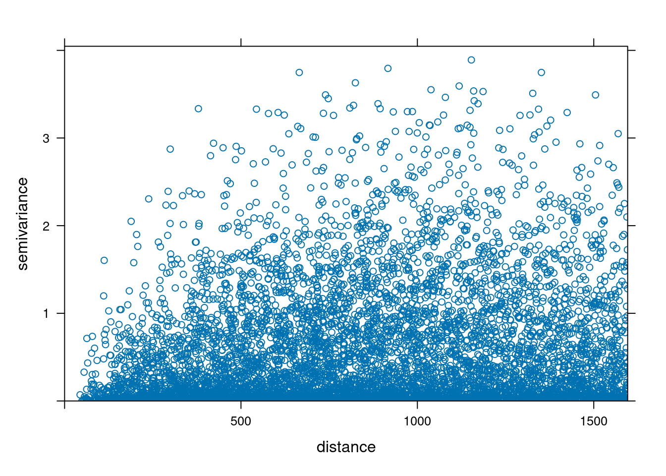
We perform a Variogram analysis to understand the spatial correlation of the zinc concentration in the dataset.

Formula: $V(h) = \frac{1}{2N(h)} \sum_{i=1}^{N(h)} (Z(s_i) - Z(s_i + h))^2$

where $V(h)$ is the semivariance at lag distance $h$, $N(h)$ is the number of pairs of observations at lag distance $h$, $Z(s_i)$ is the value of the variable at location $s_i$, and $Z(s_i + h)$ is the value of the variable at location $s_i$ plus lag distance $h$.

# Create a variogram model
vc <- variogram(log(zinc) ~ 1, meuse, cloud = TRUE)
plot(vc)

v <- variogram(log(zinc) ~ 1, meuse)
plot(v)

# Fit the variogram model
fv <- fit.variogram(object = v, 
                       model = vgm(psill = 0.5,
                                   model = "Sph", 
                                   range = 900,
                                   nugget = 0.1))
plot(v,fv)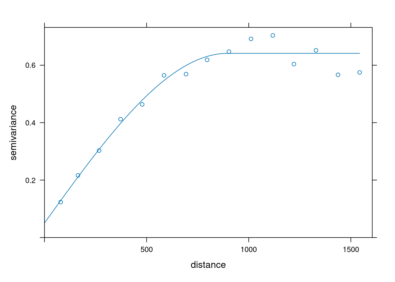

14.3.3 Perform Simple Kriging

gstat function to compute the Kriging predictions:

  `?gstat`
  

library(sf)

data(meuse)
data(meuse.grid)

meuse <- st_as_sf(meuse, 
                  coords = c("x", "y"), 
                  crs = 28992)

meuse.grid <- st_as_sf(meuse.grid, 
                       coords = c("x", "y"),
                       crs = 28992)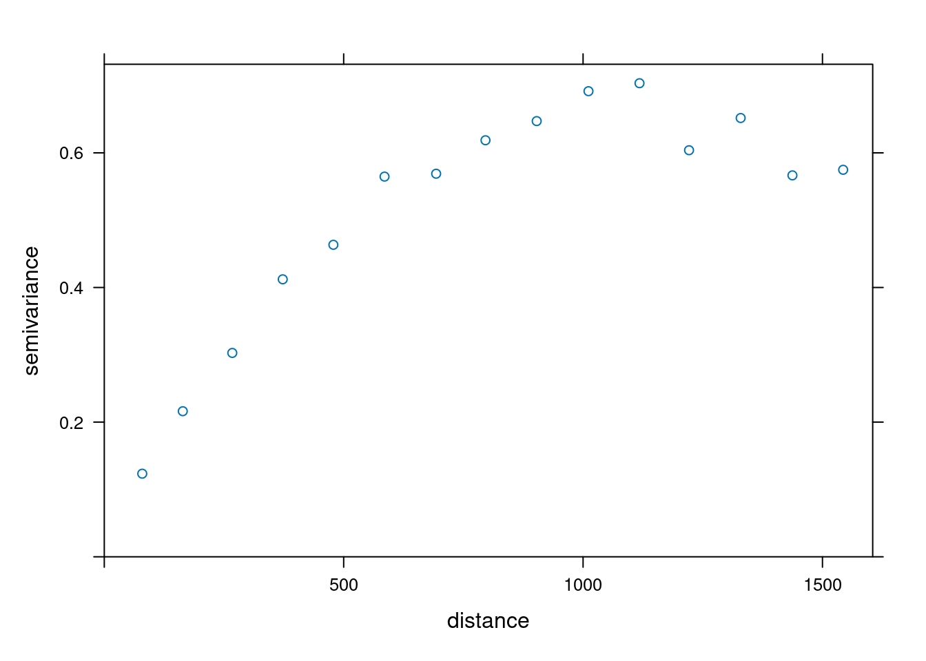

v <- variogram(log(zinc) ~ 1, meuse)
plot(v)

fv <- fit.variogram(object = v,
                    model = vgm(psill = 0.5, 
                                model = "Sph",
                                range = 900, 
                                nugget = 0.1))
fv

##   model      psill    range
## 1   Nug 0.05066017   0.0000
## 2   Sph 0.59060556 897.0044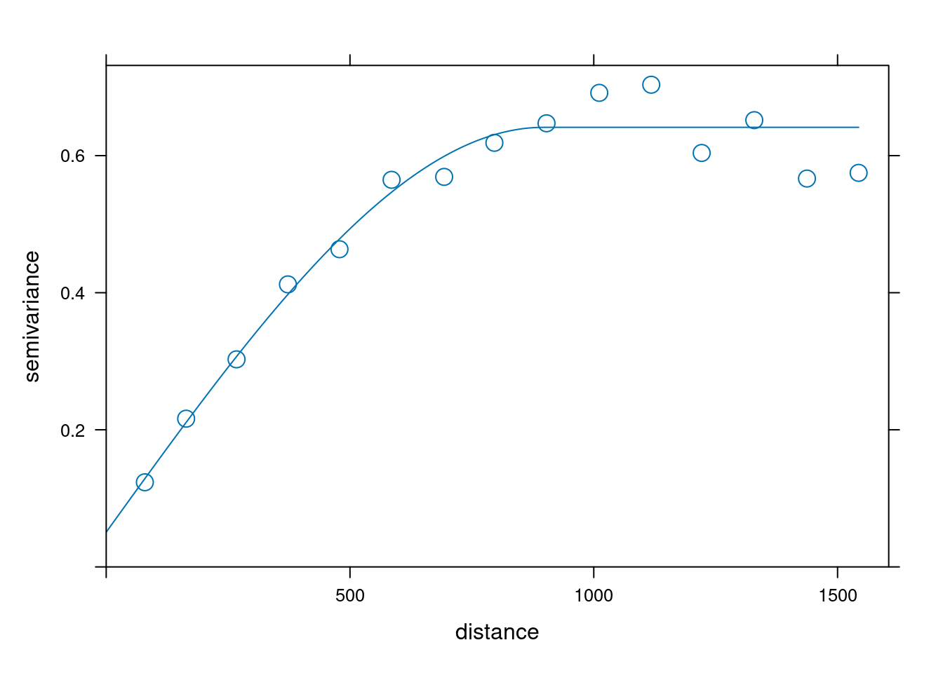

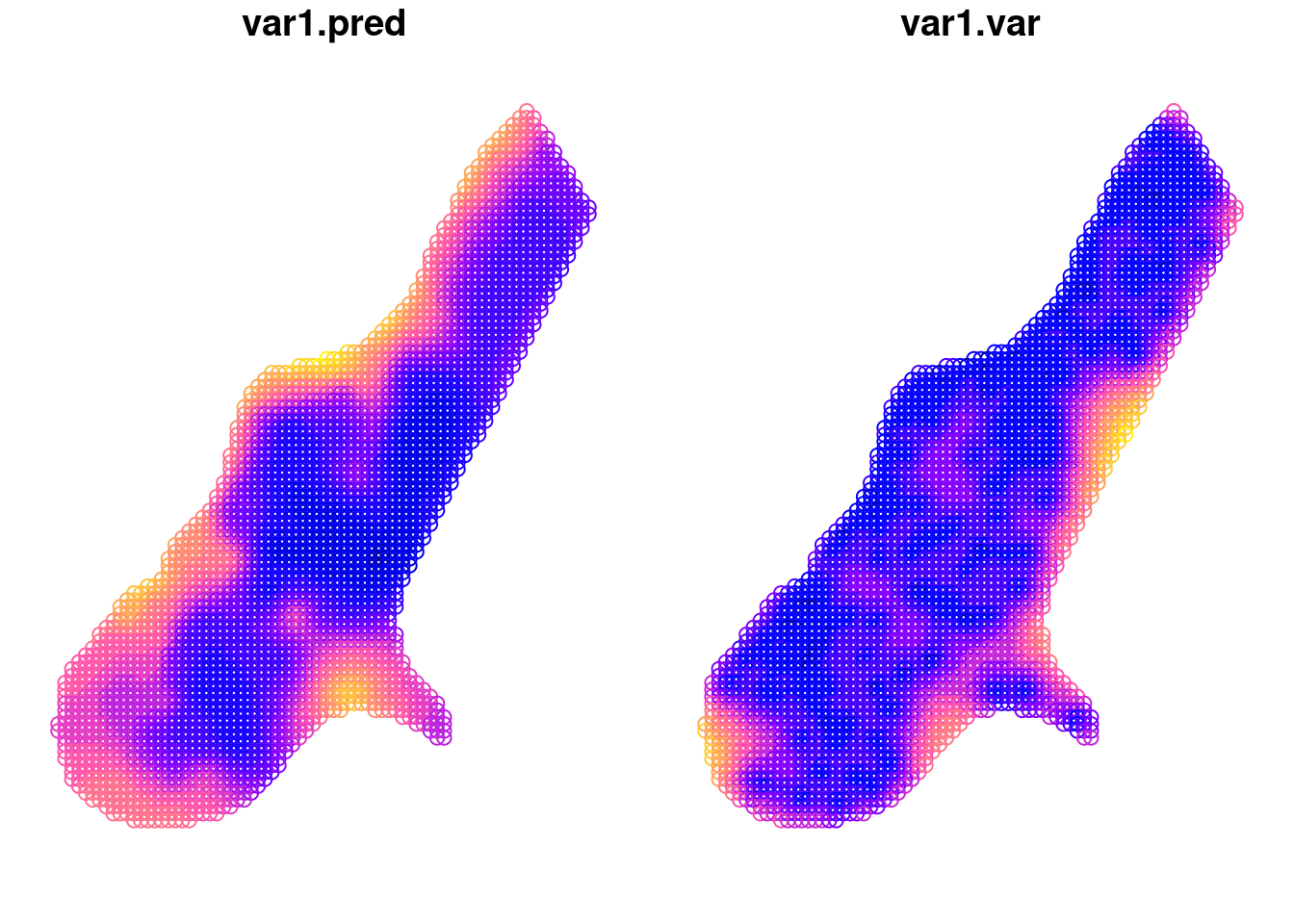
plot(v, fv, cex = 1.5)

k <- gstat(formula = log(zinc) ~ 1, 
           data = meuse, 
           model = fv)
kpred <- predict(k,meuse.grid)

## [using ordinary kriging]

ggplot() + 
  geom_sf(data = kpred, 
          aes(color = var1.pred)) +
 # geom_sf(data = meuse) +
  viridis::scale_color_viridis(name = "log(zinc)")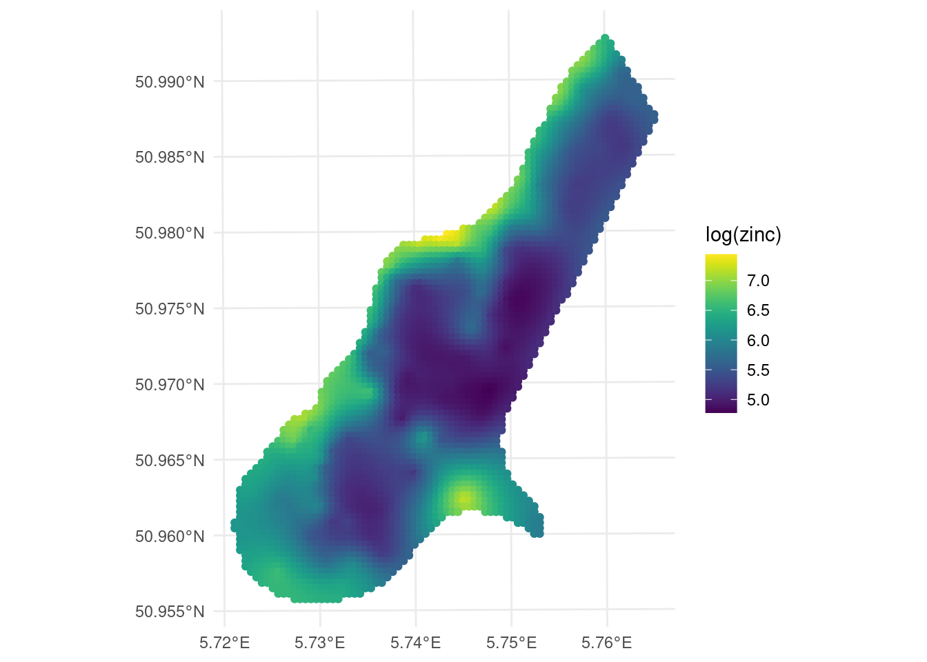

ggplot() + 
  geom_sf(data = kpred, 
          aes(color = var1.var)) +
  geom_sf(data = meuse) +
  viridis::scale_color_viridis(name = "variance")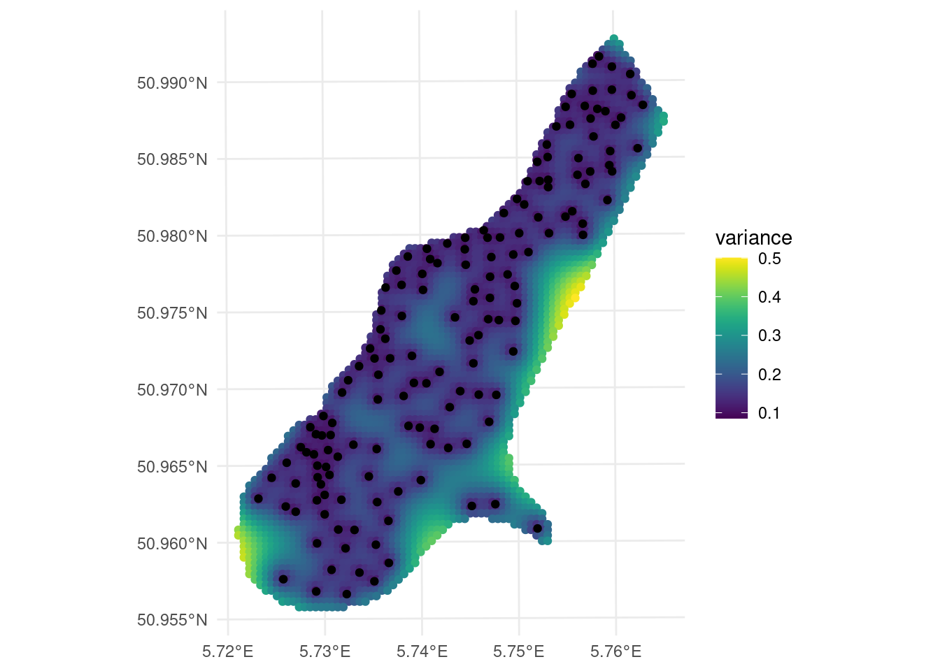 

# Perform simple Kriging
kriged <- krige(log(zinc) ~ 1, meuse,
                kpred,
                model = fv)

## [using ordinary kriging]

14.3.4 Plotting the Results

# Plot the results
plot(kriged)