Naive Bayes Example

Data: Palmer Penguins

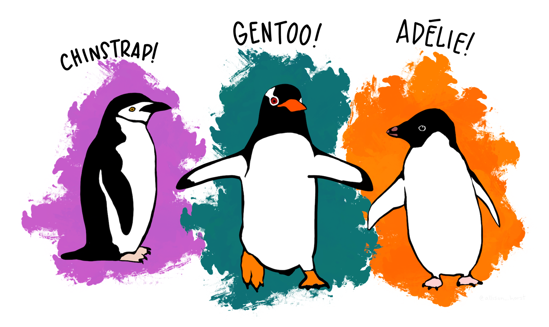
There exist multiple penguin species throughout Antarctica, including the Adelie, Chinstrap, and Gentoo. When encountering one of these penguins on an Antarctic trip, we might classify its species

$$Y = \begin{cases} A & \text{Adelie} \\ C & \text{Chinstrap} \\ G & \text{Gentoo} \end{cases}$$

three species

Example comes from chapter 14 of Bayes Rules!

Bayes Rules! textbook

$X_{1}$ categorical variable: whether the penguin weighs more than the average 4200 grams

$$X_{1} = \begin{cases} 1 & \text{above-average weight} \\ 0 & \text{below-average weight} \end{cases}$$

AKA culmen length and depth

Numerical variables:

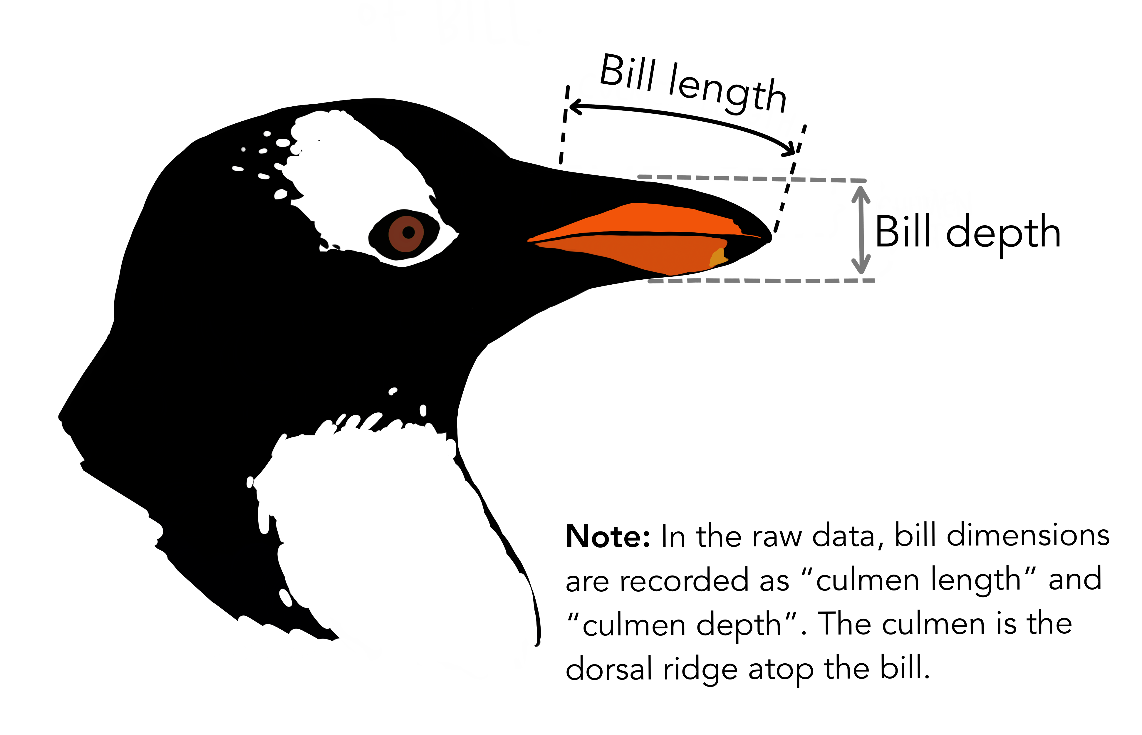
$$\begin{array}{rcl} X_{2} & = & \text{bill length (mm)} \\ X_{3} & = & \text{flipper length (mm)} \\ \end{array}$$

data(penguins_bayes)
penguins <- penguins_bayes

adelie_color = "#fb7504"
chinstrap_color = "#c65ccc"
gentoo_color = "#067476"

penguins |>
  tabyl(species)

##    species   n   percent
##     Adelie 152 0.4418605
##  Chinstrap  68 0.1976744
##     Gentoo 124 0.3604651

Motivation

Here, we have three categories, whereas logistic regression is limited to classifying binary response variables. As an alternative, naive Bayes classification

• can classify categorical response variables $Y$ with two or more categories
• doesn’t require much theory beyond Bayes’ Rule
• it’s computationally efficient, i.e., doesn’t require MCMC simulation

But why is it called “naive”?

One Categorical Predictor

Suppose an Antarctic researcher comes across a penguin that weighs less than 4200g with a 195mm-long flipper and 50mm-long bill. Our goal is to help this researcher identify the species of this penguin: Adelie, Chinstrap, or Gentoo

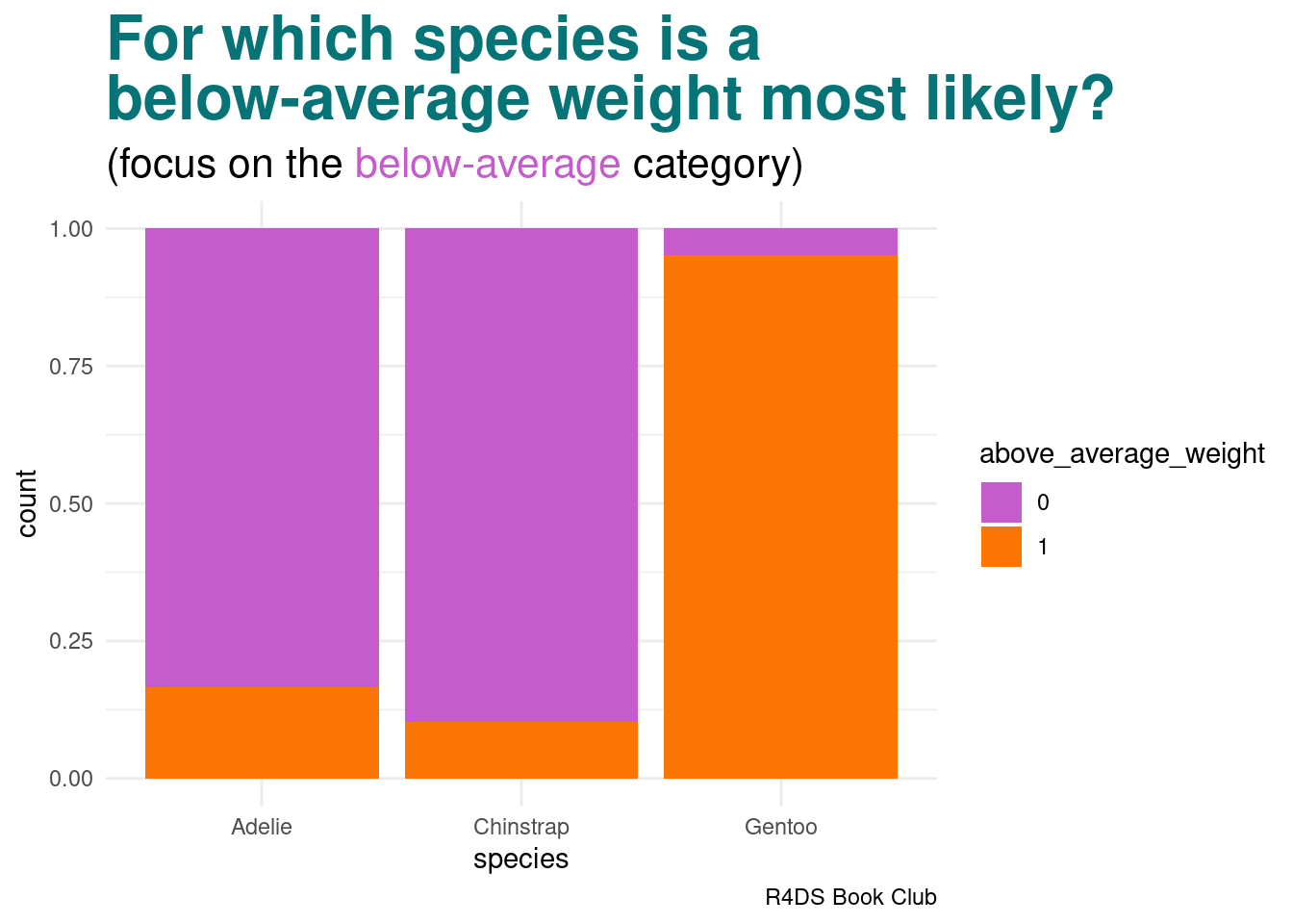
image code

penguins |>
  drop_na(above_average_weight) |>
  ggplot(aes(fill = above_average_weight, x = species)) + 
  geom_bar(position = "fill") + 
  labs(title = "<span style = 'color:#067476'>For which species is a<br>below-average weight most likely?</span>",
       subtitle = "(focus on the <span style = 'color:#c65ccc'>below-average</span> category)",
       caption = "R4DS Book Club") +
  scale_fill_manual(values = c("#c65ccc", "#fb7504")) +
  theme_minimal() +
  theme(plot.title = element_markdown(face = "bold", size = 24),
        plot.subtitle = element_markdown(size = 16))

Recall: Bayes Rule

$$f(y|x_{1}) = \frac{\text{prior}\cdot\text{likelihood}}{\text{normalizing constant}} = \frac{f(y) \cdot L(y|x_{1})}{f(x_{1})}$$ where, by the Law of Total Probability,

$$\begin{array}{rcl} f(x_{1} & = & \displaystyle\sum_{\text{all } y'} f(y')L(y'|x_{1}) \\ ~ & = & f(y' = A)L(y' = A|x_{1}) + f(y' = C)L(y' = C|x_{1}) + f(y' = G)L(y' = G|x_{1}) \\ \end{array}$$

over our three penguin species.

Calculation

penguins |> 
  select(species, above_average_weight) |> 
  na.omit() |> 
  tabyl(species, above_average_weight) |> 
  adorn_totals(c("row", "col"))

##    species   0   1 Total
##     Adelie 126  25   151
##  Chinstrap  61   7    68
##     Gentoo   6 117   123
##      Total 193 149   342

Prior probabilities:

$$f(y = A) = \frac{151}{342}, \quad f(y = C) = \frac{68}{342}, \quad f(y = G) = \frac{123}{342}$$

Likelihoods:

$$\begin{array}{rcccl} L(y = A | x_{1} = 0) & = & \frac{126}{151} & \approx & 0.8344 \\ L(y = C | x_{1} = 0) & = & \frac{61}{68} & \approx & 0.8971 \\ L(y = G | x_{1} = 0) & = & \frac{6}{123} & \approx & 0.0488 \\ \end{array}$$

Total probability:

$$f(x_{1} = 0) = \frac{151}{342}\cdot\frac{126}{151} + \frac{68}{342}\cdot\frac{61}{68} + \frac{123}{342}\cdot\frac{6}{123} = \frac{193}{342}$$

Bayes’ Rules:

$$\begin{array}{rcccccl} f(y = A | x_{1} = 0) & = & \frac{f(y = A) \cdot L(y = A | x_{1} = 0)}{f(x_{1} = 0)} = \frac{\frac{151}{342}\cdot\frac{126}{151}}{\frac{193}{342}} & \approx & 0.6528 \\ f(y = C | x_{1} = 0) & = & \frac{f(y = A) \cdot L(y = C | x_{1} = 0)}{f(x_{1} = 0)} = \frac{\frac{68}{342}\cdot\frac{61}{68}}{\frac{193}{342}} & \approx & 0.3161 \\ f(y = G | x_{1} = 0) & = & \frac{f(y = A) \cdot L(y = G | x_{1} = 0)}{f(x_{1} = 0)} = \frac{\frac{123}{342}\cdot\frac{6}{123}}{\frac{193}{342}} & \approx & 0.0311 \\ \end{array}$$

The posterior probability that this penguin is an Adelie is more than double that of the other two species

One Numerical Predictor

Let’s ignore the penguin’s weight for now and classify its species using only the fact that it has a 50mm-long bill

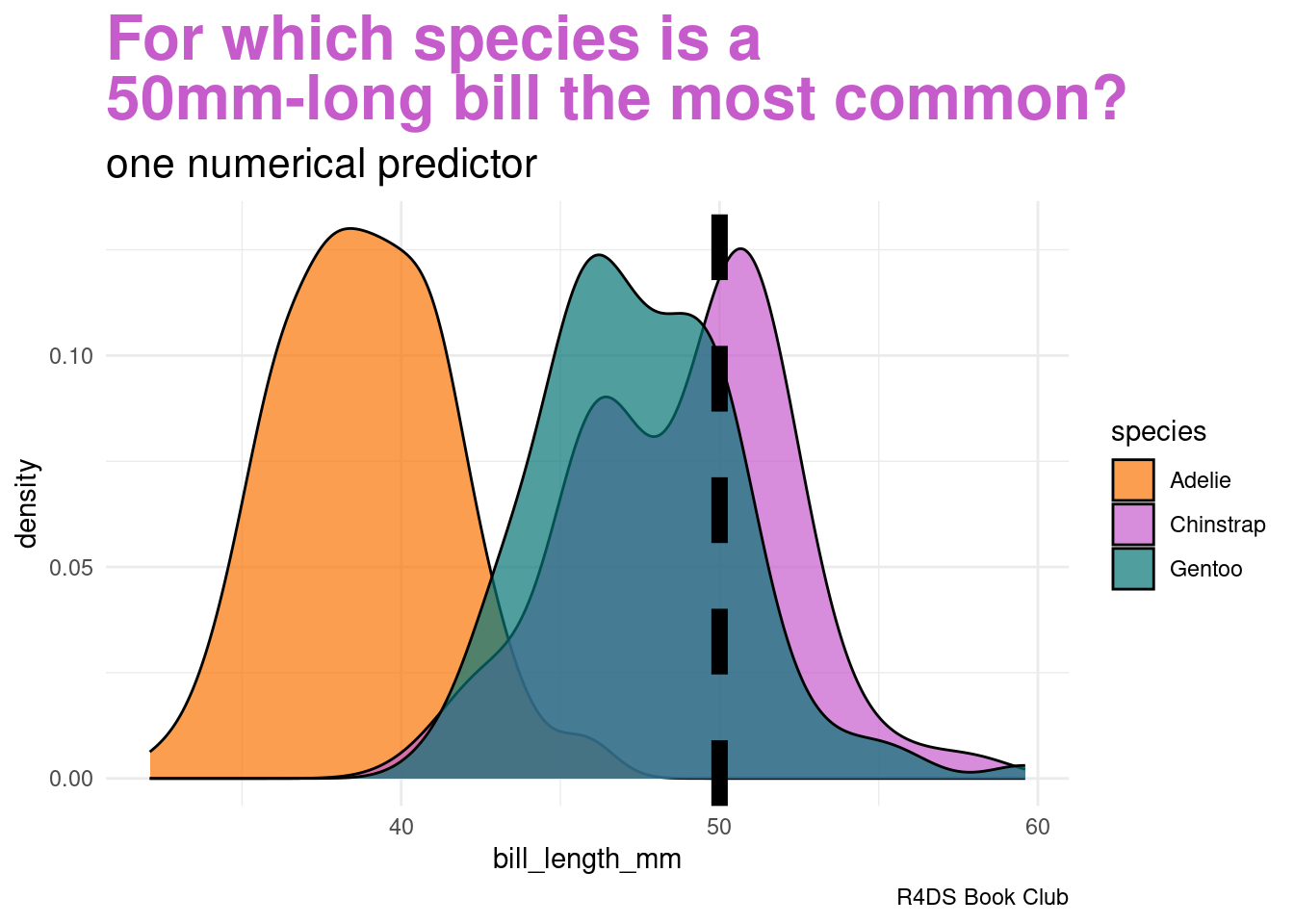
image code

penguins|>
  ggplot(aes(x = bill_length_mm, fill = species)) + 
  geom_density(alpha = 0.7) + 
  geom_vline(xintercept = 50, linetype = "dashed", linewidth = 3) + 
  labs(title = "<span style = 'color:#c65ccc'>For which species is a<br>50mm-long bill the most common?</span>",
       subtitle = "one numerical predictor",
       caption = "R4DS Book Club") +
  scale_fill_manual(values = c(adelie_color, chinstrap_color, gentoo_color)) +
  theme_minimal() +
  theme(plot.title = element_markdown(face = "bold", size = 24),
        plot.subtitle = element_markdown(size = 16))

Our data points to our penguin being a Chinstrap

• we must weigh this data against the fact that Chinstraps are the rarest of these three species
• difficult to compute likelihood $L(y = A | x_{2} = 50)$

This is where one “naive” part of naive Bayes classification comes into play. The naive Bayes method typically assumes that any quantitative predictor, here $X_{2}$, is continuous and conditionally normal:

$$\begin{array}{rcl} X_{2} | (Y = A) & \sim & N(\mu_{A}, \sigma_{A}^{2}) \\ X_{2} | (Y = C) & \sim & N(\mu_{C}, \sigma_{C}^{2}) \\ X_{2} | (Y = G) & \sim & N(\mu_{G}, \sigma_{G}^{2}) \\ \end{array}$$

Prior Probability Distributions

# Calculate sample mean and sd for each Y group
penguins |> 
  group_by(species) |> 
  summarize(mean = mean(bill_length_mm, na.rm = TRUE), 
            sd = sd(bill_length_mm, na.rm = TRUE))

## # A tibble: 3 × 3
##   species    mean    sd
##   <fct>     <dbl> <dbl>
## 1 Adelie     38.8  2.66
## 2 Chinstrap  48.8  3.34
## 3 Gentoo     47.5  3.08

penguins |>
  ggplot(aes(x = bill_length_mm, color = species)) + 
  stat_function(fun = dnorm, args = list(mean = 38.8, sd = 2.66), 
                aes(color = "Adelie"), linewidth = 3) +
  stat_function(fun = dnorm, args = list(mean = 48.8, sd = 3.34),
                aes(color = "Chinstrap"), linewidth = 3) +
  stat_function(fun = dnorm, args = list(mean = 47.5, sd = 3.08),
                aes(color = "Gentoo"), linewidth = 3) +
  ...

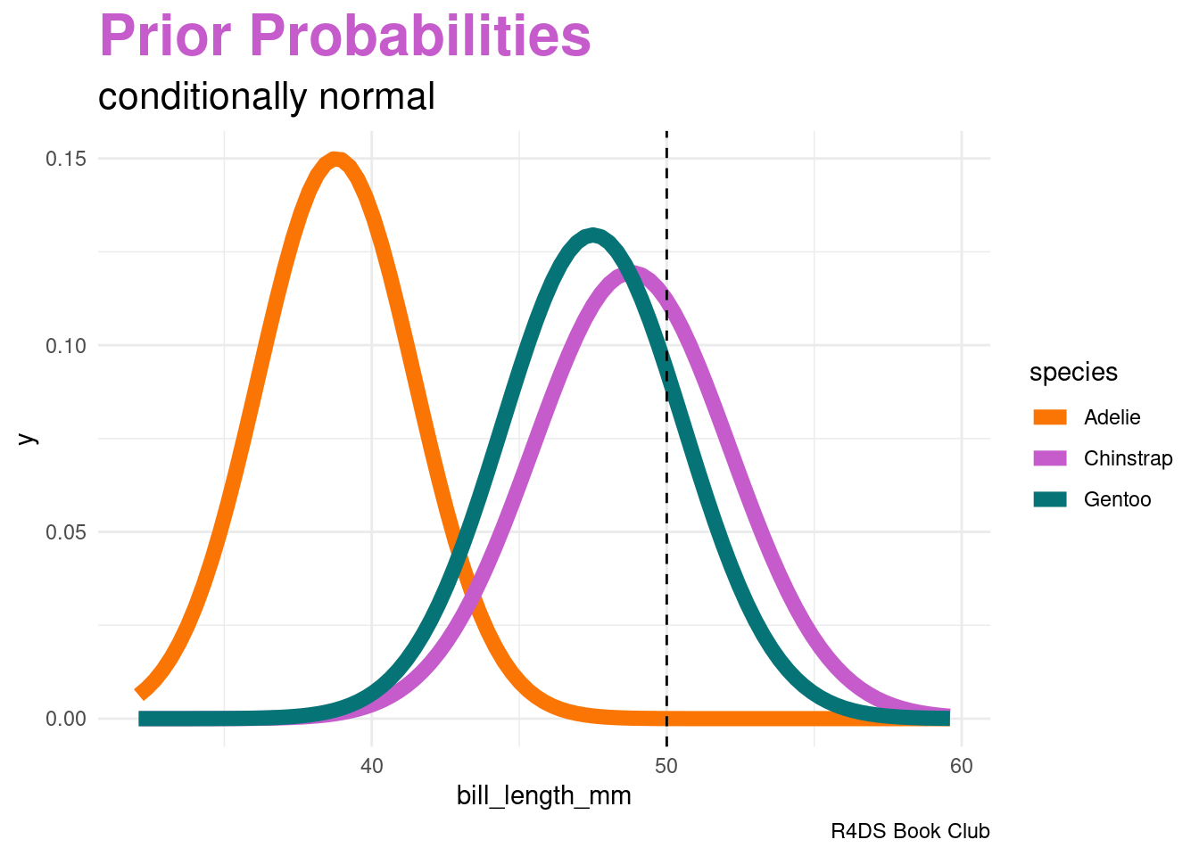
image code

penguins |>
  ggplot(aes(x = bill_length_mm, color = species)) + 
  stat_function(fun = dnorm, args = list(mean = 38.8, sd = 2.66), 
                aes(color = "Adelie"), linewidth = 3) +
  stat_function(fun = dnorm, args = list(mean = 48.8, sd = 3.34),
                aes(color = "Chinstrap"), linewidth = 3) +
  stat_function(fun = dnorm, args = list(mean = 47.5, sd = 3.08),
                aes(color = "Gentoo"), linewidth = 3) + 
  geom_vline(xintercept = 50, linetype = "dashed") + 
  labs(title = "<span style = 'color:#c65ccc'>Prior Probabilities</span>",
       subtitle = "conditionally normal",
       caption = "R4DS Book Club") +
  scale_color_manual(values = c(adelie_color, chinstrap_color, gentoo_color)) +
  theme_minimal() +
  theme(plot.title = element_markdown(face = "bold", size = 24),
        plot.subtitle = element_markdown(size = 16))

Computing the likelihoods in R:

# L(y = A | x_2 = 50) = 2.12e-05
dnorm(50, mean = 38.8, sd = 2.66)

# L(y = C | x_2 = 50) = 0.112
dnorm(50, mean = 48.8, sd = 3.34)

# L(y = G | x_2 = 50) = 0.09317
dnorm(50, mean = 47.5, sd = 3.08)

Total probability:

$$f(x_{2} = 50) = \frac{151}{342} \cdot 0.0000212 + \frac{68}{342} \cdot 0.112 + \frac{123}{342} \cdot 0.09317 \approx 0.05579$$

Bayes’ Rules:

$$\begin{array}{rcccccl} f(y = A | x_{2} = 50) & = & \frac{f(y = A) \cdot L(y = A | x_{1} = 0)}{f(x_{1} = 0)} = \frac{\frac{151}{342} \cdot 0.0000212}{0.05579} & \approx & 0.0002 \\ f(y = C | x_{2} = 50) & = & \frac{f(y = A) \cdot L(y = C | x_{1} = 0)}{f(x_{1} = 0)} = \frac{\frac{68}{342} \cdot 0.112}{0.05579} & \approx & 0.3992 \\ f(y = G | x_{2} = 50) & = & \frac{f(y = A) \cdot L(y = G | x_{1} = 0)}{f(x_{1} = 0)} = \frac{\frac{123}{342} \cdot 0.09317}{0.05579} & \approx & 0.6006 \\ \end{array}$$

Though a 50mm-long bill is relatively less common among Gentoo than among Chinstrap, it follows that our naive Bayes classification, based on our prior information and penguin’s bill length alone, is that this penguin is a Gentoo – it has the highest posterior probability.

We’ve now made two naive Bayes classifications of our penguin’s species, one based solely on the fact that our penguin has below-average weight and the other based solely on its 50mm-long bill (in addition to our prior information). And these classifications disagree: we classified the penguin as Adelie in the former analysis and Gentoo in the latter. This discrepancy indicates that there’s room for improvement in our naive Bayes classification method.

Two Predictor Variables

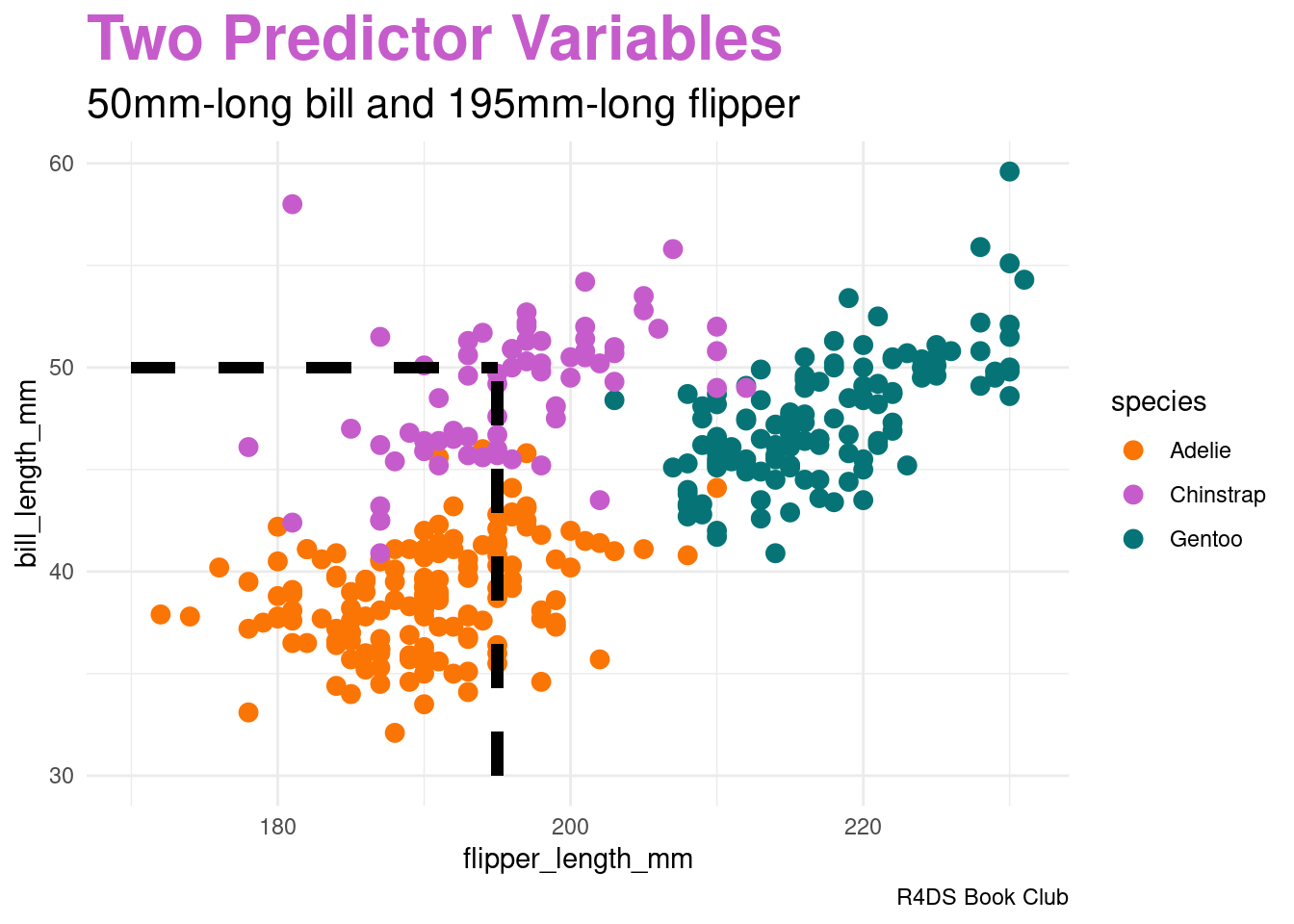
image code

penguins |>
ggplot(aes(x = flipper_length_mm, y = bill_length_mm, 
           color = species)) + 
  geom_point(size = 3) + 
  geom_segment(aes(x = 195, y = 30, xend = 195, yend = 50),
               color = "black", linetype = 2, linewidth = 2) +
  geom_segment(aes(x = 170, y = 50, xend = 195, yend = 50),
               color = "black", linetype = 2, linewidth = 2) +
  labs(title = "<span style = 'color:#c65ccc'>Two Predictor Variables</span>",
       subtitle = "50mm-long bill and 195mm-long flipper",
       caption = "R4DS Book Club") +
  scale_color_manual(values = c(adelie_color, chinstrap_color, gentoo_color)) +
  theme_minimal() +
  theme(plot.title = element_markdown(face = "bold", size = 24),
        plot.subtitle = element_markdown(size = 16))

Generalizing Bayes’ Rule:

$$f(y | x_{2}, x_{3}) = \frac{f(y) \cdot L(y | x_{2}, x_{3})}{\sum_{y'} f(y') \cdot L(y' | x_{2}, x_{3})}$$

Another “naive” assumption of conditionally independent:

$$L(y | x_{2}, x_{3}) = f(x_{2}, x_{3} | y) = f(x_{2} | y) \cdot f(x_{3} | y)$$

• mathematically efficient
• but what about correlation?

# sample statistics of x_3: flipper length
penguins |> 
  group_by(species) |> 
  summarize(mean = mean(flipper_length_mm, na.rm = TRUE), 
            sd = sd(flipper_length_mm, na.rm = TRUE))

## # A tibble: 3 × 3
##   species    mean    sd
##   <fct>     <dbl> <dbl>
## 1 Adelie     190.  6.54
## 2 Chinstrap  196.  7.13
## 3 Gentoo     217.  6.48

Likelihoods of a flipper length of 195 mm:

# L(y = A | x_3 = 195) = 0.04554
dnorm(195, mean = 190, sd = 6.54)

# L(y = C | x_3 = 195) = 0.05541
dnorm(195, mean = 196, sd = 7.13)

# L(y = G | x_3 = 195) = 0.0001934
dnorm(195, mean = 217, sd = 6.48)

Total probability:

$$f(x_{2} = 50, x_{3} = 195) = \frac{151}{342} \cdot 0.0000212 \cdot 0.04554 + \frac{68}{342} \cdot 0.112 \cdot 0.05541 + \frac{123}{342} \cdot 0.09317 \cdot 0.0001931 \approx 0.001241$$

Bayes’ Rules:

$$\begin{array}{rcccl} f(y = A | x_{2} = 50, x_{3} = 195) & = & \frac{\frac{151}{342} \cdot 0.0000212 \cdot 0.04554}{0.0001931} & \approx & 0.0003 \\ f(y = C | x_{2} = 50, x_{3} = 195) & = & \frac{\frac{68}{342} \cdot 0.112 \cdot 0.05541}{0.0001931} & \approx & 0.9944 \\ f(y = G | x_{2} = 50, x_{3} = 195) & = & \frac{\frac{123}{342} \cdot 0.09317 \cdot 0.0001931}{0.0001931} & \approx & 0.0052 \\ \end{array}$$

In conclusion, our penguin is almost certainly a Chinstrap.