MCMC

start_time <- Sys.time()

# using OLS to guide creation of prior distribution
OLS_model <- lm(bill_length_mm ~ flipper_length_mm,
                data = penguin_class_df)
OLS_intercept <- coef(OLS_model)[1]
OLS_slope     <- coef(OLS_model)[2]
mu_x <- mean(penguin_class_df$flipper_length_mm)
mu_y <- mean(penguin_class_df$bill_length_mm)
var_x <- var(penguin_class_df$flipper_length_mm)
var_y <- var(penguin_class_df$bill_length_mm)

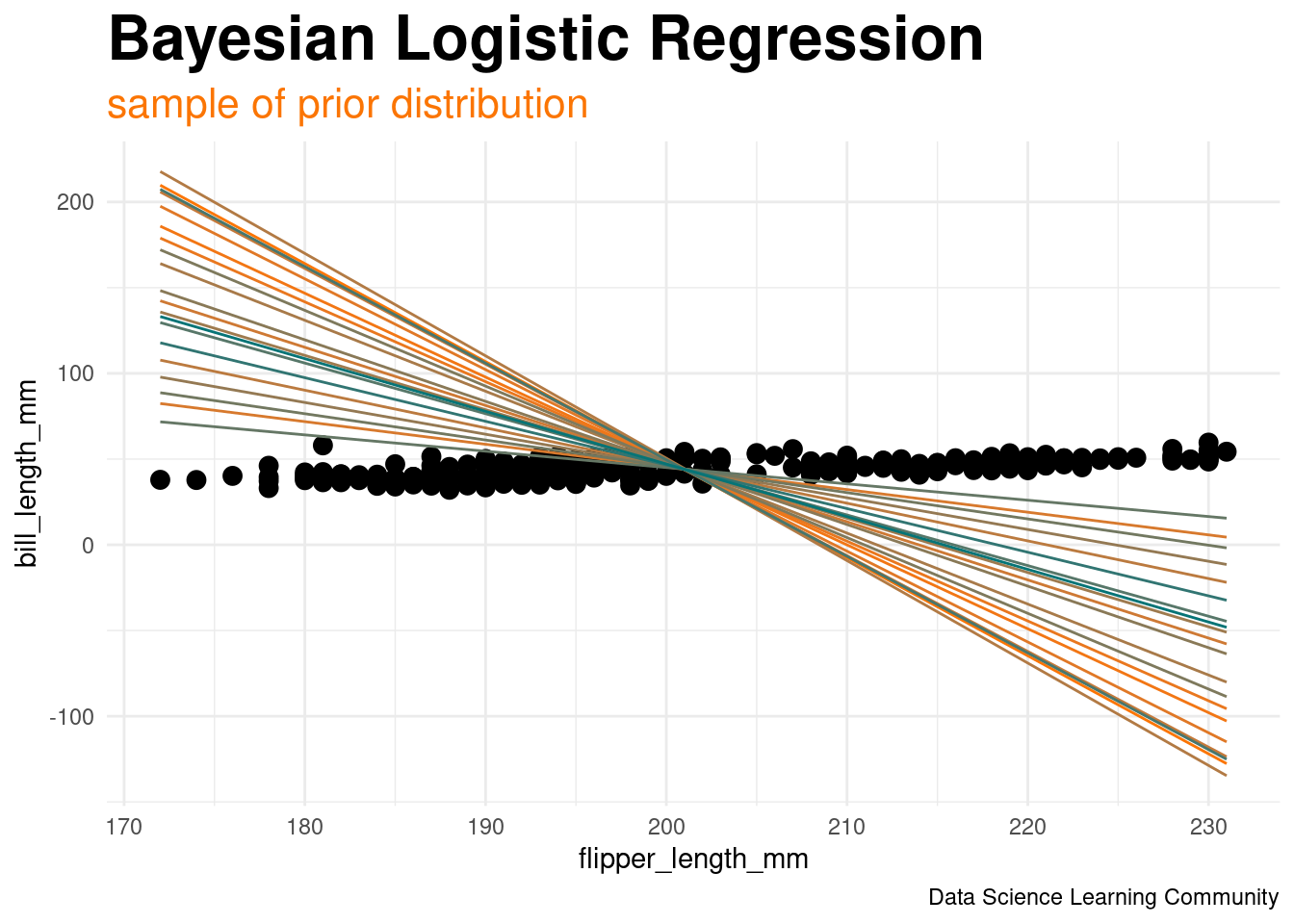
Bayesian_model_prior <- rstanarm::stan_glm(
  formula = chinstrap_bool ~ flipper_length_mm + bill_length_mm,
  data = penguin_class_df,
  family = binomial,
  prior_intercept = normal(OLS_intercept, 1),
  prior = normal(c(mu_x, mu_y), c(var_x, var_y)),
  prior_aux = exponential(1),
  prior_PD = TRUE,
  chains = 4, iter = 5000*2, refresh = 0, seed = 320)

Bayesian_model_post <- update(Bayesian_model_prior, prior_PD = FALSE)

end_time <- Sys.time()
print(end_time - start_time)

## Time difference of 20.15018 secs

Prior Distribution

R code

sim_df_prior <- as.data.frame(Bayesian_model_prior) |>
  mutate(boundary_intercept = -1.0*`(Intercept)` / bill_length_mm,
         boundary_slope = -1.0*flipper_length_mm / bill_length_mm) |>
  # grab IQR to avoid quickly ignored prior samples
  arrange(boundary_slope) |>
  slice(5000:15000)

# make data frame of line segments
flipper_min <- min(penguin_class_df$flipper_length_mm)
flipper_max <- max(penguin_class_df$flipper_length_mm)
sim_df_prior_sample <- sim_df_prior |>
  mutate(x1 = flipper_min,
         x2 = flipper_max,
         y1 = boundary_intercept + boundary_slope * x1,
         y2 = boundary_intercept + boundary_slope * x2) |>
  slice_sample(n = 20) |>
  mutate(line_id = 1:20)


# bill_min <- min(penguin_class_df$bill_length_mm)
# bill_max <- max(penguin_class_df$bill_length_mm)
penguin_class_df |>
ggplot(aes(x = flipper_length_mm, y = bill_length_mm)) + 
  geom_point(size = 3) + 
  geom_segment(aes(x = x1, y = y1, xend = x2, yend = y2,
                   color = line_id, group = line_id),
               data = sim_df_prior_sample) +
  labs(title = "Bayesian Logistic Regression",
       subtitle = "<span style = 'color:#fb7504'>sample of prior distribution</span>",
       caption = "Data Science Learning Community") +
  scale_color_gradient(low = adelie_color, high = gentoo_color) +
  theme_minimal() +
  theme(legend.position = "none",
        plot.title = element_markdown(face = "bold", size = 24),
        plot.subtitle = element_markdown(size = 16))
  # ylim(bill_min, bill_max)

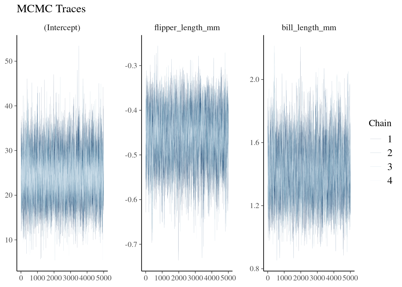
Posterior Distribution

bayesplot::mcmc_trace(Bayesian_model_post, size = 0.1) +
  labs(title = "MCMC Traces")

R code

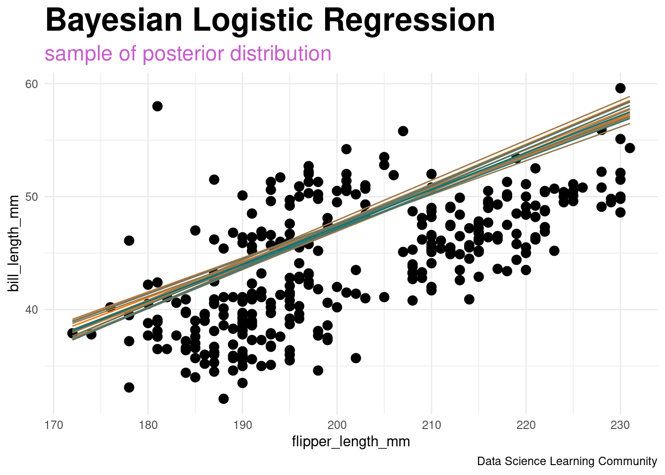
sim_df_post <- as.data.frame(Bayesian_model_post) |>
  mutate(boundary_intercept = -1.0*`(Intercept)` / bill_length_mm,
         boundary_slope = -1.0*flipper_length_mm / bill_length_mm)

# make data frame of line segments
sim_df_post_sample <- sim_df_post |>
  mutate(x1 = flipper_min,
         x2 = flipper_max,
         y1 = boundary_intercept + boundary_slope * x1,
         y2 = boundary_intercept + boundary_slope * x2) |>
  slice_sample(n = 20) |>
  mutate(line_id = 1:20)

penguin_class_df |>
ggplot(aes(x = flipper_length_mm, y = bill_length_mm)) + 
  geom_point(size = 3) + 
  geom_segment(aes(x = x1, y = y1, xend = x2, yend = y2,
                   color = line_id, group = line_id),
               data = sim_df_post_sample) +
  labs(title = "Bayesian Logistic Regression",
       subtitle = "<span style = 'color:#c65ccc'>sample of posterior distribution</span>",
       caption = "Data Science Learning Community") +
  scale_color_gradient(low = adelie_color, high = gentoo_color) +
  theme_minimal() +
  theme(legend.position = "none",
        plot.title = element_markdown(face = "bold", size = 24),
        plot.subtitle = element_markdown(size = 16))

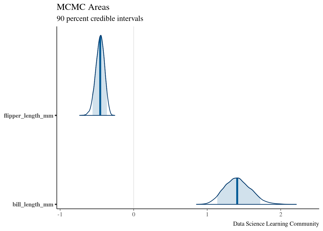
broom.mixed::tidy(Bayesian_model_post,
                  conf.int = TRUE, conf.level = 0.90) |>
  mutate_if(is.numeric, round, digits = 4)

## # A tibble: 3 × 5
##   term              estimate std.error conf.low conf.high
##   <chr>                <dbl>     <dbl>    <dbl>     <dbl>
## 1 (Intercept)         24.2      5.39     16.0      33.6  
## 2 flipper_length_mm   -0.455    0.0599   -0.559    -0.364
## 3 bill_length_mm       1.41     0.182     1.14      1.72

R code

bayesplot::mcmc_areas(Bayesian_model_post,
                      pars = c("flipper_length_mm", "bill_length_mm"),
                      prob = 0.9) +
  labs(title = "MCMC Areas",
       subtitle = "90 percent credible intervals",
       caption = "Data Science Learning Community")