Bi-Tempered Loss

R Code

penguin_class_df |>
ggplot(aes(x = flipper_length_mm, y = bill_length_mm, 
           color = chinstrap_bool)) + 
  geom_point(size = 3) +   
  geom_abline(intercept = boundary_intercept,
              slope = boundary_slope,
              color = adelie_color,
              linewidth = 2,
              linetype = 2) +
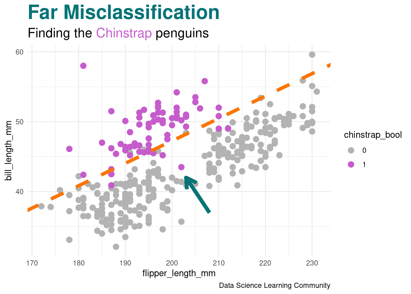
  geom_segment(aes(x = 208, y = 37, xend = 203, yend = 42),
               arrow = arrow(length = unit(0.5, "cm")),
               color = gentoo_color,
               linewidth = 2) +
  labs(title = "<span style = 'color:#067476'>Far Misclassification</span>",
       subtitle = "Finding the <span style = 'color:#c65ccc'>Chinstrap</span> penguins",
       caption = "Data Science Learning Community") +
  scale_color_manual(values = c("gray70", chinstrap_color)) +
  theme_minimal() +
  theme(plot.title = element_markdown(face = "bold", size = 24),
        plot.subtitle = element_markdown(size = 16))

With one-hot encoding and mass on class $c$, the tempered cross entropy loss is

$$L(c,\hat{y}) = \frac{1}{1 - t_{1}}\left( 1 - y_{c}^{1-t_{1}} \right) - \frac{1}{2-t_{1}}\left( 1 - \displaystyle\sum_{c'=1}^{C} \hat{y}_{c}^{2-t_{1}}\right)$$

• $0 \leq t_{1} < 1$
• As $t_{1} \rightarrow 1.0$, this reverts back to the log function and standard cross entropy

R Code

penguin_class_df |>
ggplot(aes(x = flipper_length_mm, y = bill_length_mm, 
           color = chinstrap_bool)) + 
  geom_point(size = 3) +   
  geom_abline(intercept = boundary_intercept,
              slope = boundary_slope,
              color = adelie_color,
              linewidth = 2,
              linetype = 2) +
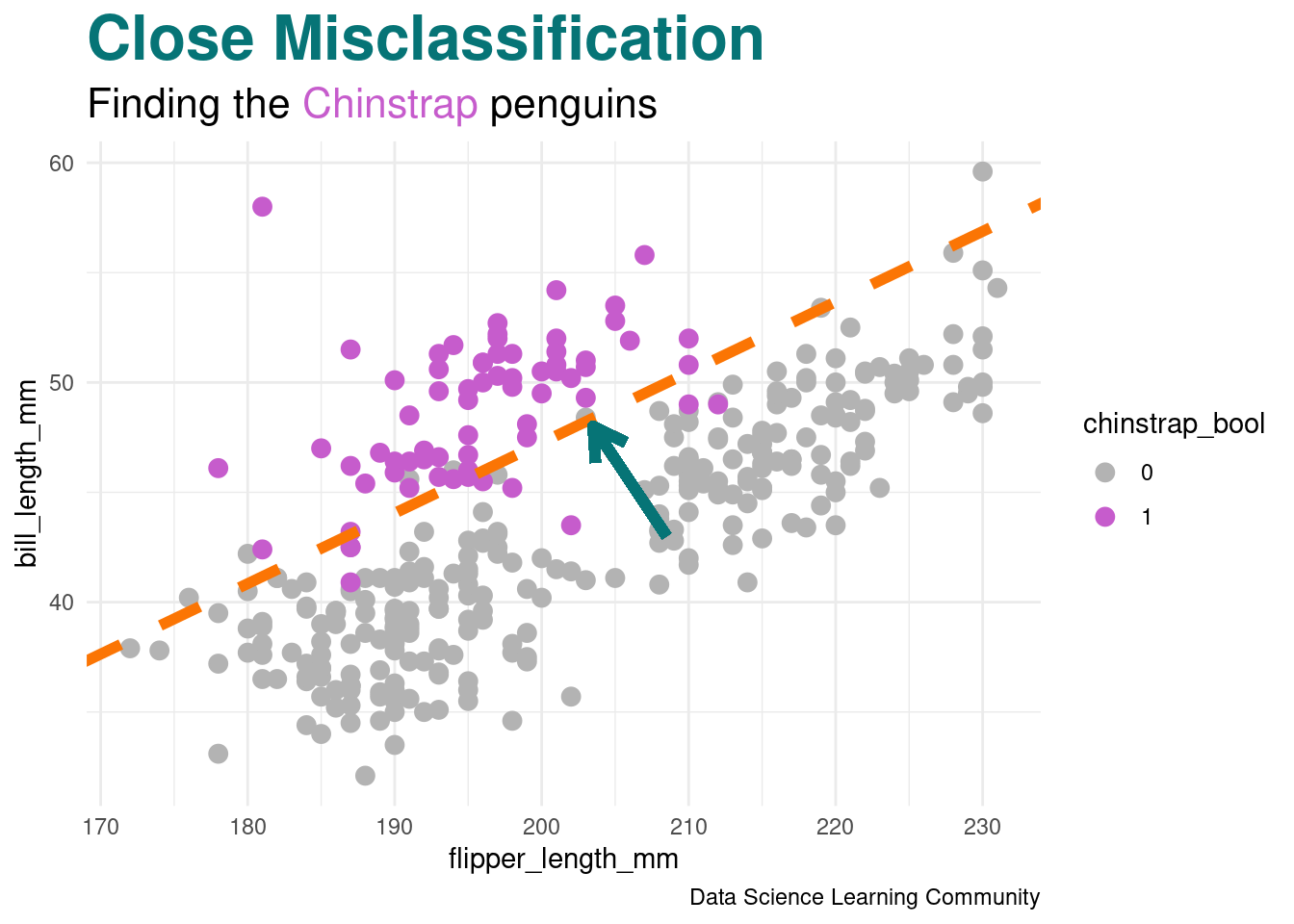
  geom_segment(aes(x = 208.5, y = 43, xend = 203.5, yend = 48),
               arrow = arrow(length = unit(0.5, "cm")),
               color = gentoo_color,
               linewidth = 2) +
  labs(title = "<span style = 'color:#067476'>Close Misclassification</span>",
       subtitle = "Finding the <span style = 'color:#c65ccc'>Chinstrap</span> penguins",
       caption = "Data Science Learning Community") +
  scale_color_manual(values = c("gray70", chinstrap_color)) +
  theme_minimal() +
  theme(plot.title = element_markdown(face = "bold", size = 24),
        plot.subtitle = element_markdown(size = 16))

The tempered softmax is

$$\hat{y}_{c} = \left[ 1 + (1-t_{2})(a_{c} - \lambda t_{2}(a)) \right]^{1/(1-t_{2})}$$

• $0 \leq t_{1} < 1 < t_{2}$

With the additional constraint $\displaystyle\sum_{c = 1}^{C} \hat{y}_{c} = 1$, we can approximate $\lambda$ with fixed-point iteration (Algorithm 10.2).