3.1 Fitting Functions to Data

Example:

year = 1955:5:2000;
temp = [ -0.0480, -0.0180, -0.0360, -0.0120, -0.0040,
       0.1180, 0.2100, 0.3320, 0.3340, 0.4560 ];
    
scatter(year,temp,label="data",
    xlabel="year",ylabel="anomaly (degrees C)",leg=:bottomright)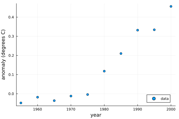

figure1

• A polynomial interpolant would overfit the data:

t = @. (year-1950)/10;
n = length(t);
V = [ t[i]^j for i in 1:n, j in 0:n-1 ];
c = V\temp;

p = Polynomial(c);
f = yr -> p((yr-1950)/10);
plot!(f,1955,2000,label="interpolant")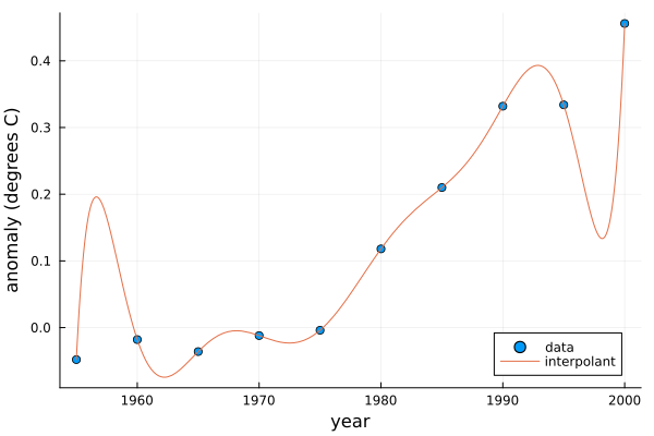

- Instead approximate with lower degree polynomial:

$$y \approx f(t) = c_1 + c_2t + \cdots + c_{n-1} t^{n-2} + c_n t^{n-1},$$ Or as matrix multiplication:

$$\begin{bmatrix} y_1 \\ y_2 \\ y_3 \\ \vdots \\ y_m \end{bmatrix} \approx \begin{bmatrix} f(t_1) \\ f(t_2) \\ f(t_3) \\ \vdots \\ f(t_m) \end{bmatrix} = \begin{bmatrix} 1 & t_1 & \cdots & t_1^{n-1} \\ 1 & t_2 & \cdots & t_2^{n-1} \\ 1 & t_3 & \cdots & t_3^{n-1} \\ \vdots & \vdots & & \vdots \\ 1 & t_m & \cdots & t_m^{n-1} \\ \end{bmatrix} \begin{bmatrix} c_1 \\ c_2 \\ \vdots \\ c_n \end{bmatrix} = \mathbf{V} \mathbf{c}.$$

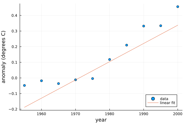
$\mathbf{V}$ is $m \times n$, taller then it is wider. We cannot solve this exactly. But Julia can solve it approximately with the same \ operator !:

V = [ t.^0 t ];
@show size(V);
c = V\temp;
p = Polynomial(c);

f = yr -> p((yr-1955)/10);
scatter(year,temp,label="data",
    xlabel="year",ylabel="anomaly (degrees C)",leg=:bottomright);
plot!(f,1955,2000,label="linear fit")

figure 3