import numpy as np # Recommended standard NumPy convention 4. NumPy Basics: Arrays and Vectorized Computation
Learning Objectives
- Learn about NumPy, a package for numerical computing in Python
- Use NumPy for array-based data: operations, algorithms
Import NumPy
Array-based operations
- A fast, flexible container for large datasets in Python
- Stores multiple items of the same type together
- Can perform operations on whole blocks of data with similar syntax
arr = np.array([[1.5, -0.1, 3], [0, -3, 6.5]])
arr
array([[ 1.5, -0.1, 3. ],
[ 0. , -3. , 6.5]])All of the elements have been multiplied by 10.
arr * 10array([[ 15., -1., 30.],
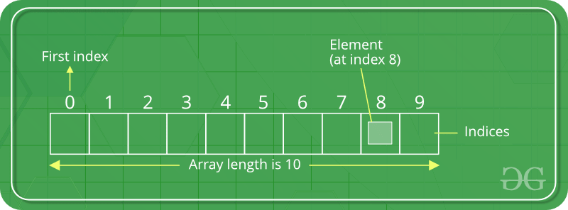
[ 0., -30., 65.]])- Every array has a
shapeindicating the size of each dimension - and a
dtype, an object describing the data type of the array
arr.shape(2, 3)arr.dtypedtype('float64')ndarray
- Generic one/multi-dimensional container where all elements are the same type
- Created using
numpy.arrayfunction
data1 = [6, 7.5, 8, 0, 1]
arr1 = np.array(data1)
arr1
array([6. , 7.5, 8. , 0. , 1. ])print(arr1.ndim)
print(arr1.shape)1
(5,)data2 = [[1, 2, 3, 4], [5, 6, 7, 8]]
arr2 = np.array(data2)
arr2array([[1, 2, 3, 4],
[5, 6, 7, 8]])print(arr2.ndim)
print(arr2.shape)2
(2, 4)Special array creation
numpy.zeroscreates an array of zeros with a given length or shapenumpy.onescreates an array of ones with a given length or shapenumpy.emptycreates an array without initialized valuesnumpy.arangecreates a range- Pass a tuple for the shape to create a higher dimensional array
np.zeros(10)array([0., 0., 0., 0., 0., 0., 0., 0., 0., 0.])np.zeros((3, 6))array([[0., 0., 0., 0., 0., 0.],
[0., 0., 0., 0., 0., 0.],
[0., 0., 0., 0., 0., 0.]])numpy.empty does not return an array of zeros, though it may look like it.
np.empty(1)array([0.])Wes provides a table of array creation functions in the book.
Data types for ndarrays
- Unless explicitly specified,
numpy.arraytries to infer a good data created arrays. - Data type is stored in a special
dtypemetadata object. - Can be explict or converted (cast)
- It is important to care about the general kind of data you’re dealing with.
arr1.dtypedtype('float64')arr2 = np.array([1, 2, 3], dtype=np.int32)
arr2.dtypedtype('int32')float_arr = arr1.astype(np.float64)
float_arr.dtypedtype('float64')int_array = arr1.astype(arr2.dtype)
int_array.dtypedtype('int32')Calling astype always creates a new array (a copy of the data), even if the new data type is the same as the old data type.
Arithmetic with NumPy Arrays
Batch operations on data without for loops
arr = np.array([[1., 2., 3.], [4., 5., 6.]])
arr * arr
array([[ 1., 4., 9.],
[16., 25., 36.]])Propagate the scalar argument to each element in the array
1 / arrarray([[1. , 0.5 , 0.33333333],
[0.25 , 0.2 , 0.16666667]])of the same size yield boolean arrays
arr2 = np.array([[0., 4., 1.], [7., 2., 12.]])

arr2 > arr
array([[False, True, False],
[ True, False, True]])Basic Indexing and Slicing
- select a subset of your data or individual elements
arr = np.arange(10)
arr
array([0, 1, 2, 3, 4, 5, 6, 7, 8, 9])Array views are on the original data. Data is not copied, and any modifications to the view will be reflected in the source array. If you want a copy of a slice of an ndarray instead of a view, you will need to explicitly copy the array—for example, arr[5:8].copy().
arr[5]5arr[5:8]array([5, 6, 7])arr[5:8] = 12Example of “not copied data”
Original
arr_slice = arr[5:8]
arr
array([ 0, 1, 2, 3, 4, 12, 12, 12, 8, 9])Change values in new array
Notice that arr is now changed.
arr_slice[1] = 123
arr
array([ 0, 1, 2, 3, 4, 12, 123, 12, 8, 9])Change all values in an array
This is done with bare slice [:]:
arr_slice[:] = 64
arr_slice
array([64, 64, 64])Higher dimensional arrays have 1D arrays at each index:
arr2d = np.array([[1,2,3], [4,5,6], [7,8,9]])
arr2d
array([[1, 2, 3],
[4, 5, 6],
[7, 8, 9]])To slice, can pass a comma-separated list to select individual elements:
arr2d[0][2]3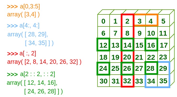
Omitting indicies will reduce number of dimensions:
arr2d[0]array([1, 2, 3])Can assign scalar values or arrays:
arr2d[0] = 9
arr2d
array([[9, 9, 9],
[4, 5, 6],
[7, 8, 9]])Or create an array of the indices. This is like indexing in two steps:
arr2d = np.array([[1,2,3], [4,5,6], [7,8,9]])
arr2d[1,0]4Indexing with slices
ndarrays can be sliced with the same syntax as Python lists:
arr = np.arange(10)

arr[1:6]
array([1, 2, 3, 4, 5])This slices a range of elements (“select the first row of arr2d”):
# arr2d[row, column]
arr2d[:1]
array([[1, 2, 3]])Can pass multiple indicies:
arr2d[:3, :1] # colons keep the dimensions
# arr2d[0:3, 0] # does not keep the dimensions
array([[1],
[4],
[7]])Boolean Indexing
names = np.array(["Bob", "Joe", "Will", "Bob", "Will", "Joe", "Joe"])
names
array(['Bob', 'Joe', 'Will', 'Bob', 'Will', 'Joe', 'Joe'], dtype='<U4')data = np.array([[4, 7], [0, 2], [-5, 6], [0, 0], [1, 2], [-12, -4], [3, 4]])
dataarray([[ 4, 7],
[ 0, 2],
[ -5, 6],
[ 0, 0],
[ 1, 2],
[-12, -4],
[ 3, 4]])Like arithmetic operations, comparisons (such as ==) with arrays are also vectorized.
names == "Bob"array([ True, False, False, True, False, False, False])This boolean array can be passed when indexing the array:
data[names == "Bob"]array([[4, 7],
[0, 0]])Select from the rows where names == “Bob” and index the columns, too:
data[names == "Bob", 1:]array([[7],
[0]])Select everything but “Bob”:
names != "Bob" # or ~(names == "Bob")array([False, True, True, False, True, True, True])Use boolean arithmetic operators like & (and) and | (or):
mask = (names == "Bob") | (names == "Will")
mask
array([ True, False, True, True, True, False, False])Selecting data from an array by boolean indexing and assigning the result to a new variable always creates a copy of the data.
Setting values with boolean arrays works by substituting the value or values on the righthand side into the locations where the boolean array’s values are True.
data[data < 0] = 0You can also set whole rows or columns using a one-dimensional boolean array:
data[names != "Joe"] = 7Fancy Indexing
A term adopted by NumPy to describe indexing using integer arrays.
arr = np.zeros((8, 4)) # 8 × 4 array

for i in range(8):
  arr[i] = i

arr
array([[0., 0., 0., 0.],
[1., 1., 1., 1.],
[2., 2., 2., 2.],
[3., 3., 3., 3.],
[4., 4., 4., 4.],
[5., 5., 5., 5.],
[6., 6., 6., 6.],
[7., 7., 7., 7.]])Pass a list or ndarray of integers specifying the desired order to subset rows in a particular order:
arr[[4, 3, 0, 6]]array([[4., 4., 4., 4.],
[3., 3., 3., 3.],
[0., 0., 0., 0.],
[6., 6., 6., 6.]])Use negative indices selects rows from the end:
arr[[-3, -5, -7]]array([[5., 5., 5., 5.],
[3., 3., 3., 3.],
[1., 1., 1., 1.]])Passing multiple index arrays selects a one-dimensional array of elements corresponding to each tuple of indices (go down then across):
arr = np.arange(32).reshape((8, 4))
arr
array([[ 0, 1, 2, 3],
[ 4, 5, 6, 7],
[ 8, 9, 10, 11],
[12, 13, 14, 15],
[16, 17, 18, 19],
[20, 21, 22, 23],
[24, 25, 26, 27],
[28, 29, 30, 31]])Here, the elements (1, 0), (5, 3), (7, 1), and (2, 2) are selected.
arr[[1, 5, 7, 2], [0, 3, 1, 2]]array([ 4, 23, 29, 10])Fancy indexing, unlike slicing, always copies the data into a new array when assigning the result to a new variable.
Transposing Arrays and Swapping Axes
Transposing is a special form of reshaping using the special T attribute:
arr = np.arange(15).reshape((3, 5))
arr
array([[ 0, 1, 2, 3, 4],
[ 5, 6, 7, 8, 9],
[10, 11, 12, 13, 14]])arr.Tarray([[ 0, 5, 10],
[ 1, 6, 11],
[ 2, 7, 12],
[ 3, 8, 13],
[ 4, 9, 14]])Matrix multiplication
np.dot(arr.T, arr)array([[125, 140, 155, 170, 185],
[140, 158, 176, 194, 212],
[155, 176, 197, 218, 239],
[170, 194, 218, 242, 266],
[185, 212, 239, 266, 293]])arr.T @ arrarray([[125, 140, 155, 170, 185],
[140, 158, 176, 194, 212],
[155, 176, 197, 218, 239],
[170, 194, 218, 242, 266],
[185, 212, 239, 266, 293]])ndarray has the method swapaxes, which takes a pair of axis numbers and switches the indicated axes to rearrange the data:
arr = np.array([[0, 1, 0], [1, 2, -2], [6, 3, 2], [-1, 0, -1], [1, 0, 1], [3, 5, 6]])
arr
arr.swapaxes(0, 1)
array([[ 0, 1, 6, -1, 1, 3],
[ 1, 2, 3, 0, 0, 5],
[ 0, -2, 2, -1, 1, 6]])Pseudorandom Number Generation
The numpy.random module supplements the built-in Python random module with functions for efficiently generating whole arrays of sample values from many kinds of probability distributions.
- Much faster than Python’s built-in
randommodule
samples = np.random.standard_normal(size=(4, 4))
samples
array([[ 0.17488936, 1.40484911, 0.15183398, -1.02194459],
[ 0.69530047, 1.69838274, -0.5782449 , -0.32245913],
[ 1.30932161, -0.48999345, -0.13171682, 0.67943756],
[-0.12637043, -0.82355441, -0.86697578, -0.06906716]])Can use an explicit generator:
seeddetermines initial state of generator
rng = np.random.default_rng(seed=12345)
data = rng.standard_normal((2, 3))
data
array([[-1.42382504, 1.26372846, -0.87066174],
[-0.25917323, -0.07534331, -0.74088465]])Wes provides a table of NumPy random number generator methods
Universal Functions: Fast Element-Wise Array Functions
A universal function, or ufunc, is a function that performs element-wise operations on data in ndarrays.
Many ufuncs are simple element-wise transformations:
One array
arr = np.arange(10)
np.sqrt(arr)
array([0. , 1. , 1.41421356, 1.73205081, 2. ,
2.23606798, 2.44948974, 2.64575131, 2.82842712, 3. ])arr1 = rng.standard_normal(10)
arr2 = rng.standard_normal(10)
np.maximum(arr1, arr2)array([ 0.78884434, 0.6488928 , 0.57585751, 1.39897899, 2.34740965,
0.96849691, 0.90291934, 0.90219827, -0.15818926, 0.44948393])remainder, whole_part = np.modf(arr1)
remainderarray([-0.3677927 , 0.6488928 , 0.36105811, -0.95286306, 0.34740965,
0.96849691, -0.75938718, 0.90219827, -0.46695317, -0.06068952])Use the out argument to assign results into an existing array rather than create a new one:
out = np.zeros_like(arr)
np.add(arr, 1, out=out)
array([ 1, 2, 3, 4, 5, 6, 7, 8, 9, 10])Array-Oriented Programming with Arrays
Evaluate the function sqrt(x^2 + y^2) across a regular grid of values: use the numpy.meshgrid function takes two one-dimensional arrays and produce two two-dimensional matrices corresponding to all pairs of (x, y) in the two arrays:
points = np.arange(-5, 5, 0.01) # 100 equally spaced points
xs, ys = np.meshgrid(points, points)
xs
array([[-5. , -4.99, -4.98, ..., 4.97, 4.98, 4.99],
[-5. , -4.99, -4.98, ..., 4.97, 4.98, 4.99],
[-5. , -4.99, -4.98, ..., 4.97, 4.98, 4.99],
...,
[-5. , -4.99, -4.98, ..., 4.97, 4.98, 4.99],
[-5. , -4.99, -4.98, ..., 4.97, 4.98, 4.99],
[-5. , -4.99, -4.98, ..., 4.97, 4.98, 4.99]])ysarray([[-5. , -5. , -5. , ..., -5. , -5. , -5. ],
[-4.99, -4.99, -4.99, ..., -4.99, -4.99, -4.99],
[-4.98, -4.98, -4.98, ..., -4.98, -4.98, -4.98],
...,
[ 4.97, 4.97, 4.97, ..., 4.97, 4.97, 4.97],
[ 4.98, 4.98, 4.98, ..., 4.98, 4.98, 4.98],
[ 4.99, 4.99, 4.99, ..., 4.99, 4.99, 4.99]])Evaluate the function as if it were two points:
z = np.sqrt(xs ** 2 + ys ** 2)
z
array([[7.07106781, 7.06400028, 7.05693985, ..., 7.04988652, 7.05693985,
7.06400028],
[7.06400028, 7.05692568, 7.04985815, ..., 7.04279774, 7.04985815,
7.05692568],
[7.05693985, 7.04985815, 7.04278354, ..., 7.03571603, 7.04278354,
7.04985815],
...,
[7.04988652, 7.04279774, 7.03571603, ..., 7.0286414 , 7.03571603,
7.04279774],
[7.05693985, 7.04985815, 7.04278354, ..., 7.03571603, 7.04278354,
7.04985815],
[7.06400028, 7.05692568, 7.04985815, ..., 7.04279774, 7.04985815,
7.05692568]])Bonus: matplotlib visualization
import matplotlib.pyplot as plt

plt.imshow(z, cmap=plt.cm.gray)  #, extent=[-25, 10, -10, 10])
plt.colorbar()
plt.title("Image plot of $\sqrt{x^2 + y^2}$ for a grid of values")
Text(0.5, 1.0, 'Image plot of $\\sqrt{x^2 + y^2}$ for a grid of values')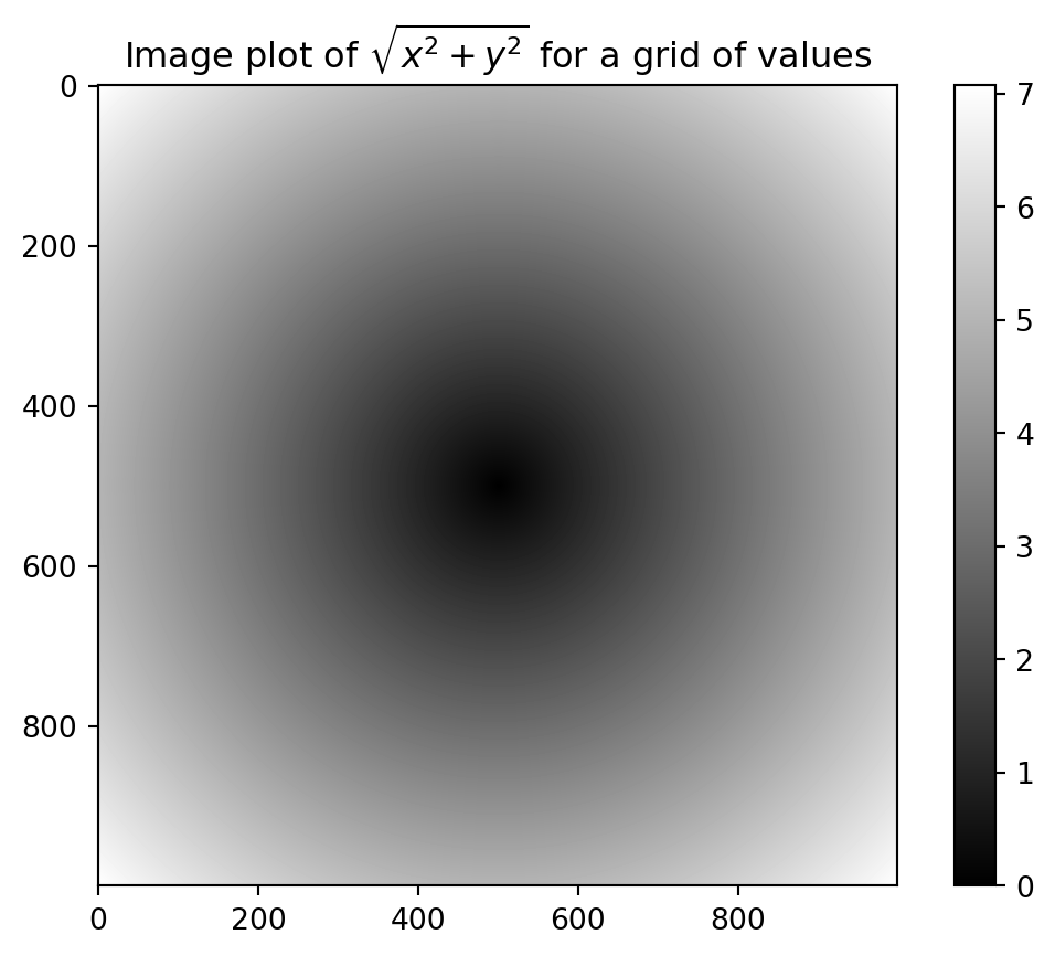
plt.close("all")Expressing Conditional Logic as Array Operations
The numpy.where function is a vectorized version of the ternary expression x if condition else.
- second and third arguments to
numpy.wherecan also be scalars - can also combine scalars and arrays
xarr = np.array([1.1, 1.2, 1.3, 1.4, 1.5])
yarr = np.array([2.1, 2.2, 2.3, 2.4, 2.5])
cond = np.array([True, False, True, True, False])
Take a value from xarr whenever the corresponding value in cond is True, and otherwise take the value from yarr:
result = [(x if c else y)
  for x, y, c in zip(xarr, yarr, cond)]

result
[1.1, 2.2, 1.3, 1.4, 2.5]result = np.where(cond, xarr, yarr)
resultarray([1.1, 2.2, 1.3, 1.4, 2.5])Can also do this with scalars, or combine arrays and scalars:
arr = rng.standard_normal((4,4))
arr
array([[-1.34360107, -0.08168759, 1.72473993, 2.61815943],
[ 0.77736134, 0.8286332 , -0.95898831, -1.20938829],
[-1.41229201, 0.54154683, 0.7519394 , -0.65876032],
[-1.22867499, 0.25755777, 0.31290292, -0.13081169]])np.where(arr > 0, 2, -2)array([[-2, -2, 2, 2],
[ 2, 2, -2, -2],
[-2, 2, 2, -2],
[-2, 2, 2, -2]])# set only positive to 2
np.where(arr > 0,2,arr)array([[-1.34360107, -0.08168759, 2. , 2. ],
[ 2. , 2. , -0.95898831, -1.20938829],
[-1.41229201, 2. , 2. , -0.65876032],
[-1.22867499, 2. , 2. , -0.13081169]])Mathematical and Statistical Methods
Use “aggregations’ like sum, mean, and std
- If using NumPy, must pass the array you want to aggregate as the first argument
arr = rng.standard_normal((5, 4))

arr.mean()0.06622379901441691np.mean(arr)0.06622379901441691Can use axis to specify which axis to computer the statistic
arr.mean(axis=1)array([ 0.00066383, 0.40377331, 0.44452789, -0.36983452, -0.14801151])arr.mean(axis=0)array([ 0.54494867, -0.10500845, 0.15080113, -0.32584615])Other methods like cumsum and cumprod do not aggregate, instead producing an array of the intermediate results:
arr.cumsum()array([1.26998312e+00, 1.17702066e+00, 1.11086977e+00, 2.65530664e-03,
1.38612157e-01, 1.48568992e+00, 1.54683394e+00, 1.61774854e+00,
2.05140308e+00, 2.32888674e+00, 2.85913913e+00, 3.39586010e+00,
4.01421011e+00, 3.21919265e+00, 3.51922360e+00, 1.91652201e+00,
2.18332084e+00, 9.21697056e-01, 8.50426250e-01, 1.32447598e+00])In multidimensional arrays, accumulation functions like cumsum compute along the indicated axis:
arr.cumsum(axis=1)array([[ 1.26998312, 1.17702066, 1.11086977, 0.00265531],
[ 0.13595685, 1.48303461, 1.54417864, 1.61509324],
[ 0.43365454, 0.7111382 , 1.24139058, 1.77811155],
[ 0.61835001, -0.17666744, 0.1233635 , -1.47933809],
[ 0.26679883, -0.99482495, -1.06609576, -0.59204603]])arr.cumsum(axis=0)array([[ 1.26998312, -0.09296246, -0.06615089, -1.10821447],
[ 1.40593997, 1.25411531, -0.00500687, -1.03729987],
[ 1.83959451, 1.53159897, 0.52524552, -0.5005789 ],
[ 2.45794452, 0.73658151, 0.82527646, -2.10328049],
[ 2.72474335, -0.52504227, 0.75400566, -1.62923076]])Methods for Boolean Arrays
Boolean values are coerced to 1 (True) and 0 (False) in the preceding methods. Thus, sum is often used as a means of counting True values in a boolean array:
(arr > 0).sum() # Number of positive values13any tests whether one or more values in an array is True, while all checks if every value is True:
bools = np.array([False, False, True, False])
bools.any()TrueSorting
NumPy arrays can be sorted in place with the sort method:
arr = rng.standard_normal(6)
arr.sort()
arr
array([-1.64041784, -1.15452958, -0.85725882, -0.41485376, 0.0977165 ,
0.68828179])Can sort multidimensional section by providing an axis:
arr = rng.standard_normal((5, 3))arr.cumsum(axis=1)array([[ 0.65045239, -0.73790756, -1.64529002],
[-1.09542531, -1.08827961, -0.55391971],
[-1.06580785, -1.24728059, 0.37467121],
[-0.31739195, -1.13320691, -0.7466279 ],
[-0.22363893, -0.92532973, -2.72104291]])arr.cumsum(axis=0)array([[ 0.65045239, -1.38835995, -0.90738246],
[-0.44497292, -1.38121426, -0.37302255],
[-1.51078076, -1.562687 , 1.24892924],
[-1.82817271, -2.37850196, 1.63550826],
[-2.05181164, -3.08019277, -0.16020491]])The top-level method numpy.sort returns a sorted copy of an array (like the Python built-in function sorted) instead of modifying the array in place:
arr2 = np.array([5, -10, 7, 1, 0, -3])
sorted_arr2 = np.sort(arr2)
sorted_arr2
array([-10, -3, 0, 1, 5, 7])Unique and Other Set Logic
numpy.unique returns the sorted unique values in an array:
np.unique(names)array(['Bob', 'Joe', 'Will'], dtype='<U4')numpy.in1d tests membership of the values in one array in another, returning a boolean array:
np.in1d(arr1, arr2)array([False, False, False, False, False, False, False, False, False,
False])File Input and Output with Arrays
NumPy is able to save np.save and load np.load data to and from disk in some text or binary formats.
Arrays are saved by default in an uncompressed raw binary format with file extension .npy:
arr = np.arange(10)
np.save("some_array", arr)np.load("some_array.npy")array([0, 1, 2, 3, 4, 5, 6, 7, 8, 9])- Save multiple arrays in an uncompressed archive using
numpy.savez - If your data compresses well, use
numpy.savez_compressedinstead
4.6 Linear Algebra
Linear algebra operations, like matrix multiplication, decompositions, determinants, and other square matrix math, can be done with Numpy (np.dot(y) vs x.dot(y)):
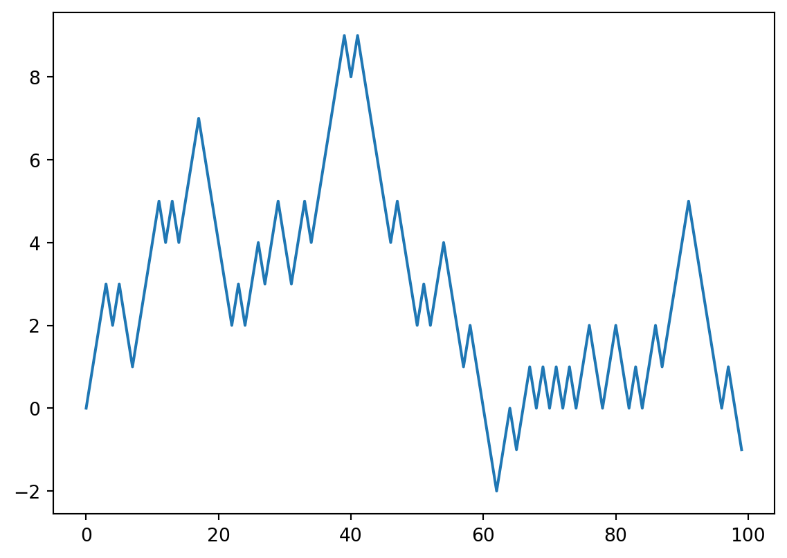
np.dot(arr1, arr)7.221776767282354Example: Random Walks
import matplotlib.pyplot as plt
#! blockstart
import random
position = 0
walk = [position]
nsteps = 1000
for _ in range(nsteps):
    step = 1 if random.randint(0, 1) else -1
    position += step
    walk.append(position)
#! blockend

plt.plot(walk[:100])
plt.show()