10.1 Sampling and Estimations
## [1] 38 15## popn persons_house house_val houses elevation poor_rate cholera_deaths
## 1 63074 5.8 207460 9370 -2 0.075 907
## 2 17208 5.8 59072 2420 0 0.143 352
## 3 50900 7.0 155175 6663 0 0.089 836
## 4 45500 6.2 107821 5674 0 0.134 734
## 5 19278 7.9 90583 2523 2 0.079 349
## 6 35227 7.1 174732 4659 2 0.076 539
## district area cholera_drate
## 1 Newington 624 144
## 2 Rotherhithe 886 205
## 3 Bermondsey 282 164
## 4 St George Southwark 688 161
## 5 St Olave 169 181
## 6 St Saviour 250 153## [1] 3810.1.1 Sample statistics
##  cholera_deaths
##  Min.   :   9.0
##  1st Qu.: 157.2
##  Median : 269.5
##  Mean   : 368.6
##  3rd Qu.: 503.2
## Max. :1618.0## # A tibble: 38 × 2
## district avg
## <chr> <dbl>
## 1 Belgrave 105
## 2 Bermondsey 836
## 3 Bethnal Green 789
## 4 Camberwell 504
## 5 Chelsea 247
## 6 Clerkenwell 121
## 7 East London 197
## 8 Greenwich 718
## 9 Hackney 139
## 10 Hammersmith, Brompton, Kensington and Fulham 225
## # ℹ 28 more rowscholera%>%#names
ggplot(aes(cholera_deaths))+
geom_density()+
geom_vline(aes(xintercept=mean(cholera_deaths)),
color="red",linewidth=0.5)+
geom_text(aes(x=mean(cholera_deaths)+100,y=0.0015,
label="Mean"))+
geom_vline(aes(xintercept=sd(cholera_deaths)),
color="darkred",linewidth=0.5)+
geom_text(aes(x=mean(cholera_deaths)-100,y=0.0010,
label="SD"))+
ggthemes::theme_fivethirtyeight()## Warning in geom_text(aes(x = mean(cholera_deaths) + 100, y = 0.0015, label = "Mean")): All aesthetics have length 1, but the data has 38 rows.
## ℹ Did you mean to use `annotate()`?## Warning in geom_text(aes(x = mean(cholera_deaths) - 100, y = 0.001, label = "SD")): All aesthetics have length 1, but the data has 38 rows.
## ℹ Did you mean to use `annotate()`?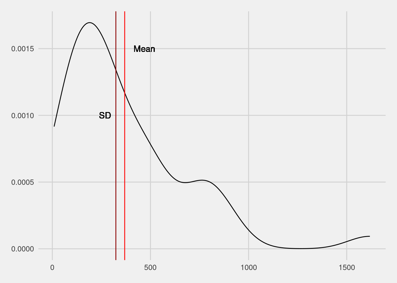
cholera%>%#names
  ggplot(aes(x=cholera_deaths,fill=water))+
    geom_histogram(position="stack",
                   bins=10,color="white")+
  labs(x="Deaths")+
  ggthemes::scale_fill_fivethirtyeight()+
  ggthemes::theme_fivethirtyeight()+
  theme(axis.title.x = element_text())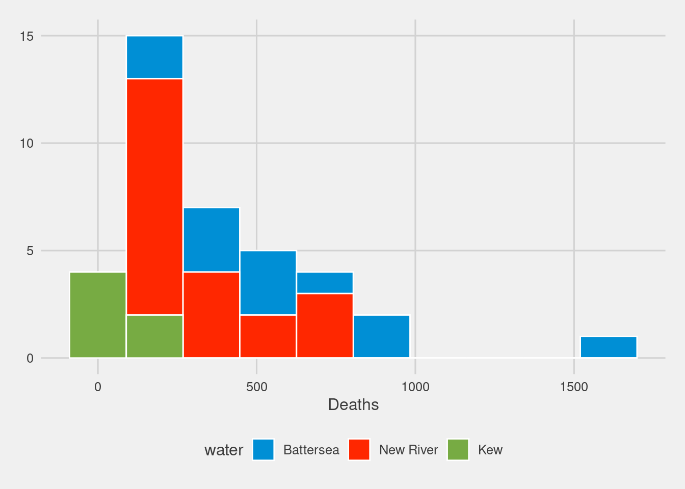
10.1.2 The IQ example
IQ <- rnorm(n = 10000, mean = 100, sd = 15) # generate IQ scores
IQ <- round(IQ) # IQs are whole numbers!
head(IQ)
## [1] 94 97 68 114 96 99To make this with ggplot2:
- geom_histogram(aes(y=..density..), position=“stack”, fill=“steelblue”, bins=30,color=“white”)
- stat_function(fun = dnorm, color=“green”, args = list(mean = mean(IQ), sd = sd(IQ)))
## # A tibble: 10,000 × 2
##       IQ    dist
##    <dbl>   <dbl>
##  1    94 0.0244
##  2    97 0.0260
##  3    68 0.00273
##  4   114 0.0173
##  5    96 0.0255
##  6    99 0.0264
##  7   117 0.0141
##  8    94 0.0244
##  9   108 0.0231
## 10   107 0.0238
## # ℹ 9,990 more rows## IQ dist
## Min. : 45.0 Min. :2.666e-05
## 1st Qu.: 90.0 1st Qu.:1.392e-02
## Median :100.0 Median :2.118e-02
## Mean :100.1 Mean :1.872e-02
## 3rd Qu.:110.0 3rd Qu.:2.513e-02
## Max. :156.0 Max. :2.651e-02## `stat_bin()` using `bins = 30`. Pick better value with `binwidth`.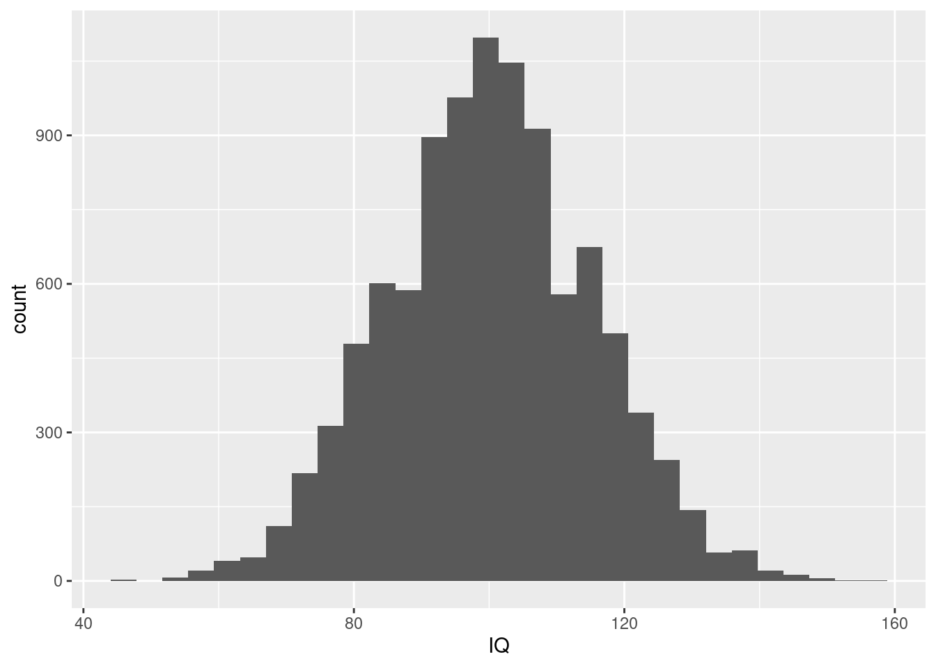
##
## Call:
##  density.default(x = IQ)
##
## Data: IQ (10000 obs.);   Bandwidth 'bw' = 2.129
##
##        x                y
##  Min.   : 38.61   Min.   :2.210e-07
##  1st Qu.: 69.56   1st Qu.:2.476e-04
##  Median :100.50   Median :3.345e-03
##  Mean   :100.50   Mean   :8.071e-03
##  3rd Qu.:131.44   3rd Qu.:1.550e-02
## Max. :162.39 Max. :2.670e-02tibble(IQ)%>%#names
ggplot(aes(x=IQ))+
geom_histogram(aes(y =..density..),
#position="stack",
fill="steelblue",
bins=30,
color="white")+
stat_function(fun = dnorm,
color="green",
args = list(mean = mean(IQ), sd = sd(IQ)))+
geom_vline(aes(xintercept=mean(IQ)),
color="red",linewidth=0.5)+
geom_text(aes(x=mean(IQ)+10,y=0.02,
label="Mean"))+
ggthemes::scale_fill_fivethirtyeight()+
ggthemes::theme_fivethirtyeight()## Warning: The dot-dot notation (`..density..`) was deprecated in ggplot2 3.4.0.
## ℹ Please use `after_stat(density)` instead.
## This warning is displayed once every 8 hours.
## Call `lifecycle::last_lifecycle_warnings()` to see where this warning was
## generated.## Warning in geom_text(aes(x = mean(IQ) + 10, y = 0.02, label = "Mean")): All aesthetics have length 1, but the data has 10000 rows.
## ℹ Did you mean to use `annotate()`?
tibble(IQ=sample(IQ,size = 10000*3,replace = T))%>%#names
  ggplot(aes(x=IQ))+
  geom_histogram(aes(y=..density..),
                 position="stack",
                   fill="steelblue",
                   bins=30,color="white")+
 stat_function(fun = dnorm,
               color="green",
               args = list(mean = mean(IQ), sd = sd(IQ)))+
  geom_vline(aes(xintercept=mean(IQ)),
             color="red",linewidth=0.5)+
  geom_text(aes(x=mean(IQ)+10,y=0.02,
                label="Mean"))+
  ggthemes::scale_fill_fivethirtyeight()+
  ggthemes::theme_fivethirtyeight()
## Warning in geom_text(aes(x = mean(IQ) + 10, y = 0.02, label = "Mean")): All aesthetics have length 1, but the data has 30000 rows.
## ℹ Did you mean to use `annotate()`?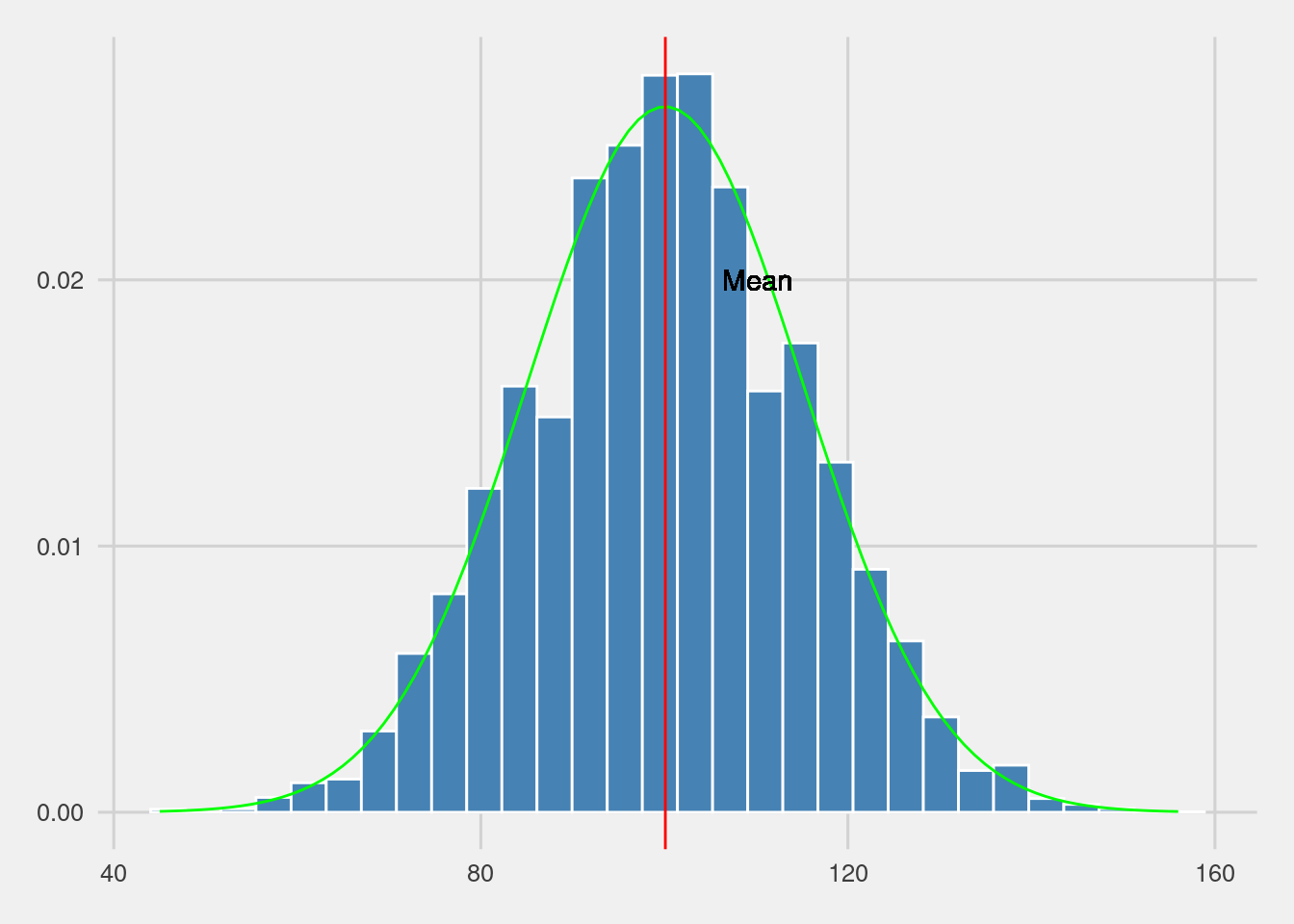
width <- 6
    height <- 6

# parameters of the beta
    a <- 2
    b <- 1

# mean and standard deviation of the beta
    s <- sqrt( a*b / (a+b)^2 / (a+b+1) )
    m <- a / (a+b)
# define function to draw a plot
plotOne <- function(n,N=50000) {
# generate N random sample means of size n
X <- matrix(rbeta(n*N,a,b),n,N)
X <- colMeans(X)
# plot the data
hist( X, breaks=seq(0,1,.025), border="white", freq=FALSE,
col="grey",
xlab="Sample Mean", ylab="", xlim=c(0,1.2),
main=paste("Sample Size =",n), axes=FALSE,
font.main=1, ylim=c(0,5)
)
box()
axis(1)
#axis(2)
# plot the theoretical distribution
lines( x <- seq(0,1.2,.01), dnorm(x,m,s/sqrt(n)),
lwd=2, col="black", type="l"
)
}
for( i in c(1,2,4,8)) {
plotOne(i)}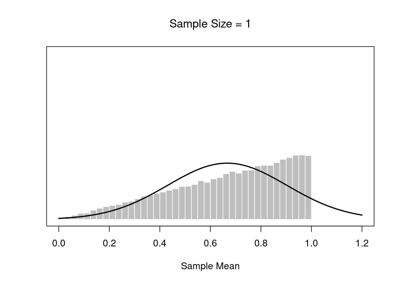
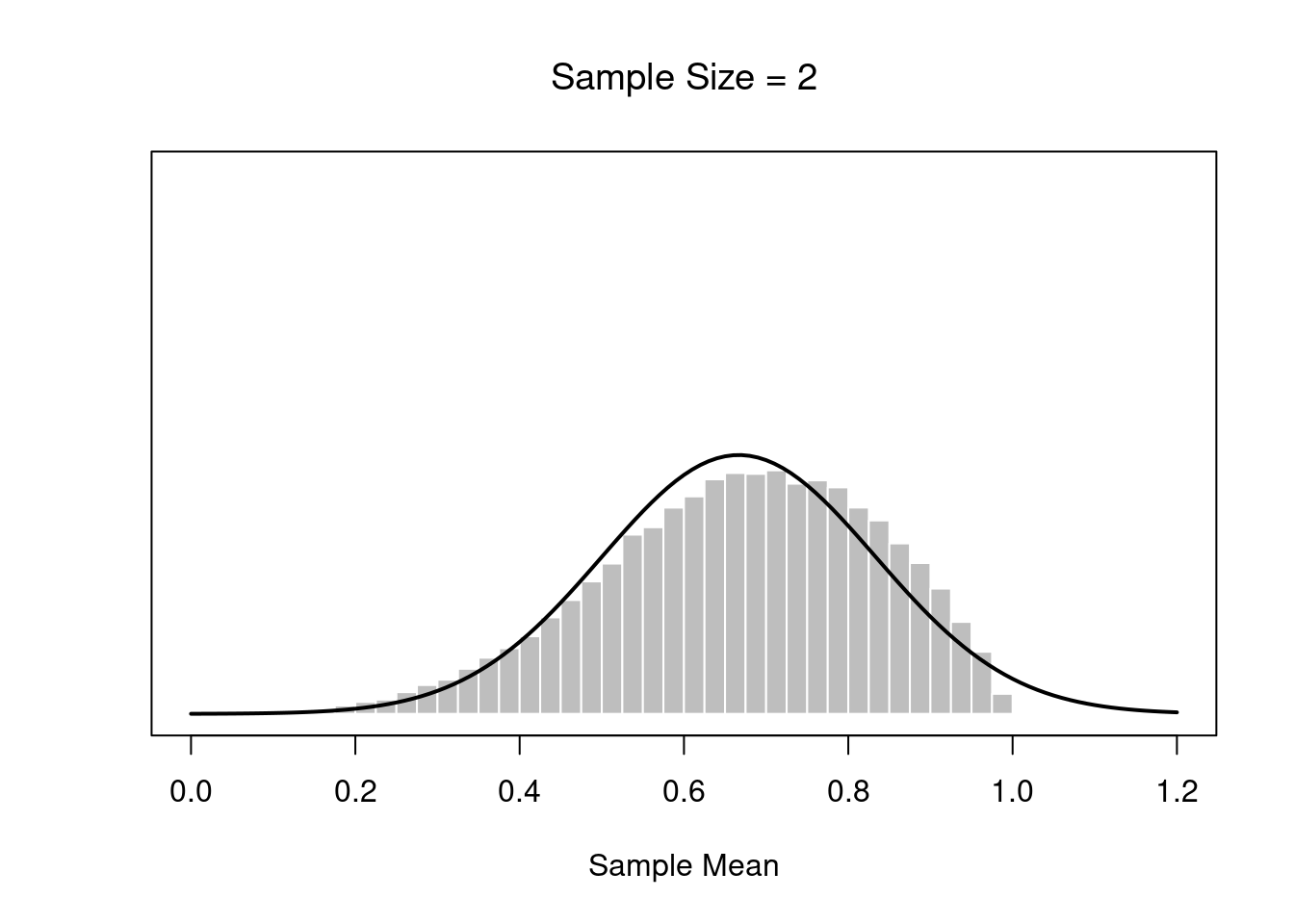
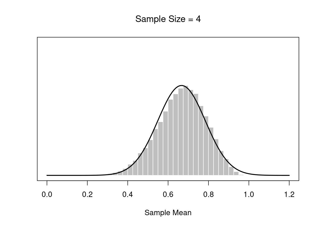
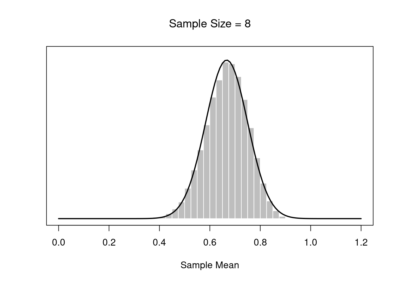
If the population distribution has mean \(\mu\) and standard deviation \(\sigma\), then the sampling distribution of the mean also has mean \(\mu\), and the standard error of the mean is: \[SEM=\frac{\sigma}{\sqrt(N)}\]