11.4 Evaluate the results of a statistical hypothesis testing

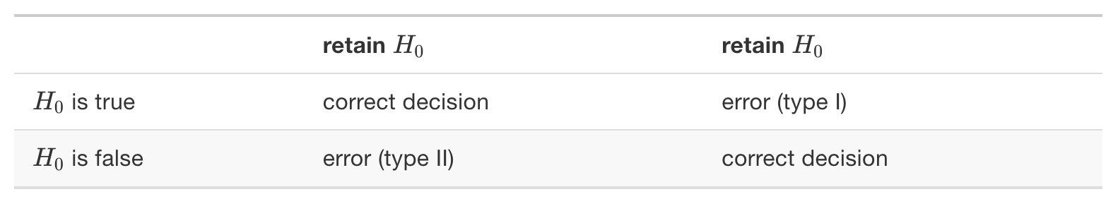
Type I and Type II errors

11.4.0.1 Case Study: medical diagnostic test

Suppose we have a new medical test designed to detect a particular disease, and we want to assess its accuracy.

Scenario:

Null Hypothesis (H0): The patient does not have the disease
Alternative Hypothesis (Ha): The patient has the disease

Simulate test results for two groups: patients without the disease and patients with the disease. Then, perform a hypothesis test based on the test results and evaluate Type I and Type II errors.

Simulate data

set.seed(123)

True disease status (0 for no disease, 1 for disease)

population_without_disease <- rbinom(1000, size = 1, prob = 0.1)
population_with_disease <- rbinom(1000, size = 1, prob = 0.8)

population_without_disease

##    [1] 0 0 0 0 1 0 0 0 0 0 1 0 0 0 0 0 0 0 0 1 0 0 0 1 0 0 0 0 0 0 1 1 0 0 0 0 0
##   [38] 0 0 0 0 0 0 0 0 0 0 0 0 0 0 0 0 0 0 0 0 0 0 0 0 0 0 0 0 0 0 0 0 0 0 0 0 0
##   [75] 0 0 0 0 0 0 0 0 0 0 0 0 1 0 0 0 0 0 0 0 0 0 0 0 0 0 0 0 0 1 0 0 1 0 0 0 1
##  [112] 0 0 1 0 0 0 1 0 0 0 0 0 0 0 1 0 0 0 0 0 0 0 0 0 0 0 0 1 0 0 0 0 0 0 0 0 0
##  [149] 0 0 0 0 0 0 0 0 0 0 0 0 0 0 0 0 0 0 0 0 0 0 0 0 0 0 0 0 0 0 0 0 0 0 0 0 0
##  [186] 0 0 0 1 1 0 0 1 0 1 0 0 0 0 0 0 1 0 0 0 0 0 0 0 0 0 0 0 0 0 0 0 0 0 1 0 1
##  [223] 0 0 0 0 0 0 0 1 0 0 0 0 0 0 0 0 0 0 0 0 0 0 0 0 0 1 1 0 0 0 0 0 0 0 0 0 0
##  [260] 0 1 0 0 1 0 0 0 0 0 0 0 0 0 0 0 0 1 0 0 0 0 0 0 0 0 0 0 0 0 0 0 0 0 0 0 0
##  [297] 1 0 0 0 0 0 0 0 0 0 0 0 0 0 0 0 0 0 0 0 0 0 0 0 0 0 0 0 0 0 1 0 0 1 0 0 0
##  [334] 0 0 0 0 0 0 1 0 0 0 0 0 0 1 0 0 0 0 1 0 0 0 1 0 0 0 0 0 0 0 0 0 0 0 0 0 0
##  [371] 0 0 0 0 0 1 0 0 0 1 0 0 0 0 0 1 0 0 0 0 1 0 0 0 0 0 0 0 0 1 1 0 1 0 0 0 0
##  [408] 0 0 0 0 0 0 0 0 0 1 0 0 0 0 0 0 0 0 0 0 0 0 0 1 0 0 1 0 0 0 0 0 0 0 0 0 0
##  [445] 0 0 0 0 0 0 0 0 0 0 0 0 0 0 0 0 1 0 0 0 0 0 0 0 0 0 0 0 0 0 0 0 0 0 0 0 0
##  [482] 0 0 0 1 0 0 0 0 0 1 0 0 0 0 1 0 0 0 0 0 0 0 0 0 0 0 0 1 0 0 0 0 0 0 0 0 0
##  [519] 0 0 0 0 0 0 0 0 1 0 1 0 1 0 0 0 0 0 0 0 0 0 0 0 0 0 0 1 0 0 0 0 0 0 0 0 0
##  [556] 0 0 0 0 0 0 1 0 0 0 0 0 0 0 0 0 1 0 0 1 0 0 0 0 0 0 0 0 0 0 0 0 0 1 0 0 0
##  [593] 1 0 0 0 0 0 0 0 0 0 0 0 0 0 0 0 0 0 0 0 0 1 0 0 0 0 1 0 1 0 0 0 0 0 0 0 0
##  [630] 0 0 0 0 0 0 0 1 0 0 0 0 0 0 0 0 0 0 0 0 0 0 1 0 0 0 0 1 0 0 0 0 0 0 0 0 0
##  [667] 1 0 0 0 0 0 0 0 0 0 0 0 0 0 0 0 0 0 1 0 0 0 0 0 0 0 0 0 0 0 0 0 0 0 0 0 0
##  [704] 0 0 0 0 0 0 0 0 0 0 0 0 0 0 0 1 0 0 0 0 0 0 0 0 0 0 0 0 0 0 1 0 0 0 1 0 0
##  [741] 1 0 0 0 0 0 0 0 0 1 0 0 0 0 0 0 0 0 0 0 0 0 0 0 0 0 0 0 0 0 1 0 0 0 0 0 0
##  [778] 0 0 0 0 0 0 0 0 0 0 0 0 1 1 0 0 0 0 0 0 0 0 0 0 0 0 0 0 1 0 0 0 0 0 0 0 0
##  [815] 0 0 0 0 0 0 0 0 0 1 0 0 0 0 0 0 0 0 0 0 0 0 0 0 0 0 1 0 0 0 0 0 0 0 0 0 0
##  [852] 0 1 0 0 0 1 0 0 0 0 0 0 0 0 0 0 0 0 0 0 0 0 0 0 0 0 0 0 0 0 1 0 0 0 1 0 0
##  [889] 0 0 0 0 0 0 0 0 0 0 0 0 1 0 0 0 0 0 0 1 0 0 0 0 0 0 0 1 0 0 0 0 0 0 0 0 0
##  [926] 0 0 0 0 0 0 0 0 0 1 0 0 0 0 0 1 0 0 0 0 0 0 0 0 0 0 0 1 0 0 1 0 0 0 0 0 0
##  [963] 0 0 1 0 0 0 0 0 0 0 0 0 0 0 1 0 0 0 0 0 1 0 1 0 0 0 0 0 0 0 0 0 0 0 0 0 0
## [1000] 0

Assuming a Type I error rate (α) of 0.05 and a Type II error rate (β) of 0.2

alpha <- 0.05
beta <- 0.2

test_results_without_disease <- rbinom(1000, size = 1, prob = alpha) * (1 - population_without_disease)

test_results_with_disease <- rbinom(1000, size = 1, prob = 1 - beta) * population_with_disease

11.4.0.1.1 Hypothesis testing

result <- t.test(test_results_with_disease, test_results_without_disease)
result

## 
##  Welch Two Sample t-test
## 
## data:  test_results_with_disease and test_results_without_disease
## t = 35.436, df = 1325.7, p-value < 2.2e-16
## alternative hypothesis: true difference in means is not equal to 0
## 95 percent confidence interval:
##  0.553559 0.618441
## sample estimates:
## mean of x mean of y 
##     0.627     0.041

11.4.0.1.2 Determine Type I and Type II errors

cutoff <- qnorm(1 - alpha)

# Calculate the critical value for a Type I error

True positive: Patients with the disease correctly identified

true_positive <- sum(test_results_with_disease == 1)

False positive: Patients without the disease incorrectly identified as having it

false_positive <- sum(test_results_without_disease == 1)

True negative: Patients without the disease correctly identified as not having it

true_negative <- sum(test_results_without_disease == 0)

False negative: Patients with the disease incorrectly identified as not having it

false_negative <- sum(test_results_with_disease == 0)

Calculate Type I and Type II error rates

type_i_error_rate <- false_positive / (false_positive + true_negative)
type_ii_error_rate <- false_negative / (false_negative + true_positive)

cat("Type I Error Rate (False Positive Rate):", type_i_error_rate, "\n")

## Type I Error Rate (False Positive Rate): 0.041

cat("Type II Error Rate (False Negative Rate):", type_ii_error_rate, "\n")

## Type II Error Rate (False Negative Rate): 0.373