1.3 Example 1: Tidying the works of Jane Austen

Loading the texts and converting it into a tibble data format:

library(janeaustenr)
library(dplyr)
library(stringr)

original_books <- austen_books() %>%
  group_by(book) %>%
  mutate(linenumber = row_number(),
         chapter = cumsum(str_detect(text, 
                                     regex("^chapter [\\divxlc]",
                                           ignore_case = TRUE)))) %>%
  ungroup()

original_books

## # A tibble: 73,422 × 4
##    text                    book                linenumber chapter
##    <chr>                   <fct>                    <int>   <int>
##  1 "SENSE AND SENSIBILITY" Sense & Sensibility          1       0
##  2 ""                      Sense & Sensibility          2       0
##  3 "by Jane Austen"        Sense & Sensibility          3       0
##  4 ""                      Sense & Sensibility          4       0
##  5 "(1811)"                Sense & Sensibility          5       0
##  6 ""                      Sense & Sensibility          6       0
##  7 ""                      Sense & Sensibility          7       0
##  8 ""                      Sense & Sensibility          8       0
##  9 ""                      Sense & Sensibility          9       0
## 10 "CHAPTER 1"             Sense & Sensibility         10       1
## # … with 73,412 more rows

Restructuring the one-token-per-row tidytext data format:

library(tidytext)
tidy_books <- original_books %>%
  unnest_tokens(word, text)

tidy_books

## # A tibble: 725,055 × 4
##    book                linenumber chapter word       
##    <fct>                    <int>   <int> <chr>      
##  1 Sense & Sensibility          1       0 sense      
##  2 Sense & Sensibility          1       0 and        
##  3 Sense & Sensibility          1       0 sensibility
##  4 Sense & Sensibility          3       0 by         
##  5 Sense & Sensibility          3       0 jane       
##  6 Sense & Sensibility          3       0 austen     
##  7 Sense & Sensibility          5       0 1811       
##  8 Sense & Sensibility         10       1 chapter    
##  9 Sense & Sensibility         10       1 1          
## 10 Sense & Sensibility         13       1 the        
## # … with 725,045 more rows

Removing the stopwords: Often in text analysis, we will want to remove stop words; stop words are words that are not useful for an analysis, typically extremely common words such as “the”, “of”, “to”, and so forth in English. We can remove stop words (kept in the tidytext dataset stop_words) with an anti_join().

data(stop_words)

tidy_books <- tidy_books %>%
  anti_join(stop_words)

## Joining, by = "word"

We can use them all together, as we have here, or filter() to only use one set of stop words if that is more appropriate for a certain analysis.

Using the dplyr::count() to summarize the word frequency results as a tidy data table:

tidy_books %>%
  count(word, sort = TRUE) 

## # A tibble: 13,914 × 2
##    word       n
##    <chr>  <int>
##  1 miss    1855
##  2 time    1337
##  3 fanny    862
##  4 dear     822
##  5 lady     817
##  6 sir      806
##  7 day      797
##  8 emma     787
##  9 sister   727
## 10 house    699
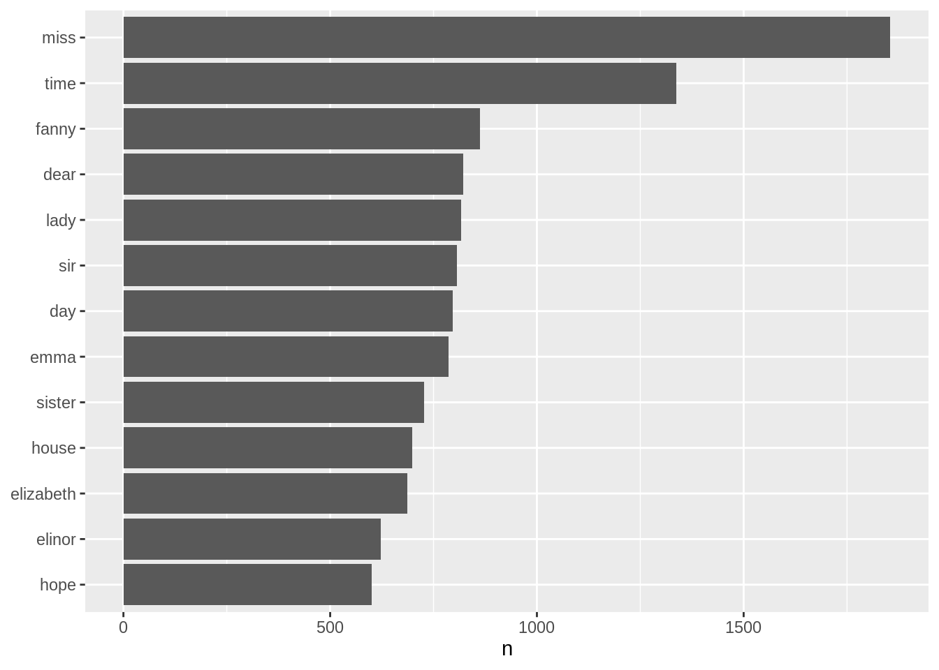
## # … with 13,904 more rows

Visualizing the word frequency results as a plot:

library(ggplot2)

tidy_books %>%
  count(word, sort = TRUE) %>%
  filter(n > 600) %>%
  mutate(word = reorder(word, n)) %>%
  ggplot(aes(n, word)) +
  geom_col() +
  labs(y = NULL)