# Notes {-}
## Introduction: Tree-based methods
- Involve **stratifying** or **segmenting** the predictor space into a number of simple regions
- Are simple and useful for interpretation
- However, basic decision trees are NOT competitive with the best supervised learning approaches in terms of prediction accuracy
- Thus, we also discuss **bagging**, **random forests**, and **boosting** (i.e., tree-based ensemble methods) to grow multiple trees which are then combined to yield a single consensus prediction
- These can result in dramatic improvements in prediction accuracy (but some loss of interpretability)
- Can be applied to both regression and classification
## Regression Trees
First, let's take a look at `Hitters` dataset.
```{r}
#| label: 08-hitters-dataset
#| echo: false
library(dplyr)
library(tidyr)
library(readr)
df <- read_csv('./data/Hitters.csv') %>%
select(Names, Hits, Years, Salary) %>%
drop_na() %>%
mutate(log_Salary = log(Salary))
df
```
```{r}
#| label: 08-reg-trees-intro
#| echo: false
#| out-width: 100%
knitr::include_graphics("images/08_1_salary_data.png")
knitr::include_graphics("images/08_2_basic_tree.png")
```
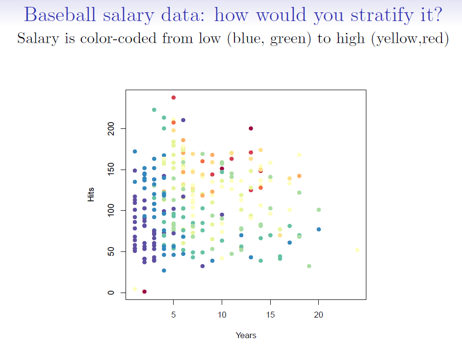
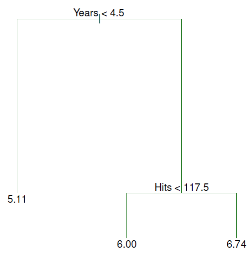
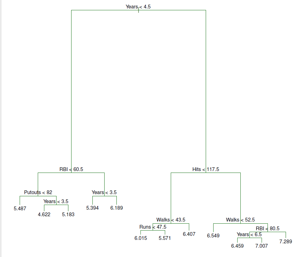
- For the Hitters data, a regression tree for predicting the log salary of a baseball player based on:
1. number of years that he has played in the major leagues
2. number of hits that he made in the previous year
## Terminology
```{r}
#| label: 08-decision-trees-terminology-1
#| echo: false
#| out-width: 100%
knitr::include_graphics("images/08_3_basic_tree_term.png")
```
```{r}
#| label: 08-decision-trees-terminology-2
#| echo: false
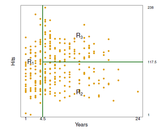
#| fig-cap: The three-region partition for the Hitters data set from the regression tree
#| out-width: 100%
knitr::include_graphics("images/08_4_hitters_predictor_space.png")
```
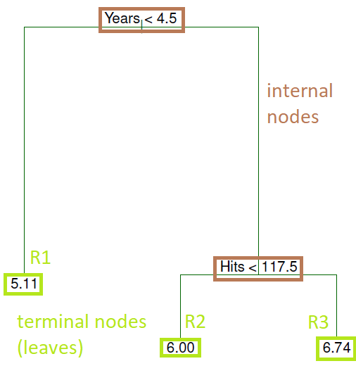
- Overall, the tree stratifies or segments the players into three regions of predictor space:
- R1 = {X \| Years\< 4.5}
- R2 = {X \| Years\>=4.5, Hits\<117.5}
- R3 = {X \| Years\>=4.5, Hits\>=117.5}
where R1, R2, and R3 are **terminal nodes** (leaves) and green lines (where the predictor space is split) are the **internal nodes**
- The number in each leaf/terminal node is the mean of the response for the observations that fall there
## Interpretation of results: regression tree (Hitters data)
```{r}
#| label: 08-reg-trees-interpreration
#| echo: false
#| out-width: 100%
knitr::include_graphics("images/08_2_basic_tree.png")
```
1. `Years` is the most important factor in determining `Salary`: players with less experience earn lower salaries than more experienced players
2. Given that a player is less experienced, the number of `Hits` that he made in the previous year seems to play little role in his `Salary`
3. But among players who have been in the major leagues for 5 or more years, the number of Hits made in the previous year does affect Salary: players who made more Hits last year tend to have higher salaries
4. This is surely an over-simplification, but compared to a regression model, it is easy to display, interpret and explain
## Tree-building process (regression)
1. Divide the predictor space --- that is, the set of possible values for $X_1,X_2, . . . ,X_p$ --- into $J$ distinct and **non-overlapping** regions, $R_1,R_2, . . . ,R_J$
- Regions can have ANY shape - they don't have to be boxes
2. For every observation that falls into the region $R_j$, we make the same prediction: the **mean** of the response values in $R_j$
3. The goal is to find regions (here boxes) $R_1, . . . ,R_J$ that **minimize** the $RSS$, given by
$$\mathrm{RSS}=\sum_{j=1}^{J}\sum_{i{\in}R_j}^{}(y_i - \hat{y}_{R_j})^2$$
where $\hat{y}_{R_j}$ is the **mean** response for the training observations within the $j$th box
- Unfortunately, it is **computationally infeasible** to consider every possible partition of the feature space into $J$ boxes.
## Recursive binary splitting
So, take a top-down, greedy approach known as recursive binary splitting:
- **top-down** because it begins at the top of the tree and then successively splits the predictor space
- **greedy** because at each step of the tree-building process, the best split is made at that particular step, rather than looking ahead and picking a split that will lead to a better tree in some future step
1. First, select the predictor $X_j$ and the cutpoint $s$ such that splitting the predictor space into the regions ${\{X|X_j<s\}}$ and ${\{X|X_j{\ge}s}\}$ leads to the greatest possible reduction in RSS
2. Repeat the process looking for the best predictor and best cutpoint to split data further (i.e., split one of the 2 previously identified regions - not the entire predictor space) minimizing the RSS within each of the resulting regions
3. Continue until a stopping criterion is reached, e.g., no region contains more than five observations
4. Again, we predict the response for a given test observation using the **mean of the training observations** in the region to which that test observation belongs
but ...
- The previous method may result in a tree that **overfits** the data. Why?
- Tree is too leafy (complex)
- A better strategy is to have a smaller tree with fewer splits, which will reduce variance and lead to better interpretation of results (at the cost of a little bias)
- So we will prune
## Pruning a tree
1. Grow a very large tree $T_0$ as before
2. Apply cost-complexity pruning to $T_0$ to obtain a sequence of BEST subtrees, as a function of $\alpha$
Cost complexity pruning minimizes (Eq. 8.4)
$\sum_{m=1}^{|T|}\sum_{x_i{\in}R_m}(y_i-\hat{y}_{R_m})^2 + \alpha|T|$
where
$\alpha$ $\geq$ 0
$|T|$ is the number of **terminal nodes** the sub tree $|T|$ holds
$R_m$ is the rectangle/region (i.e., the subset of predictor space) corresponding to the $m$th terminal node
$\hat{y}_{R_m}$ is the **mean** response for the training observations in $R_m$
- the tuning parameter $\alpha$ controls:
a. a trade-off between the subtree's complexity (the number of terminal nodes)
b. the subtree's fit to the training data
3. Choose $\alpha$ using K-fold cross-validation
- repeat steps 1) and 2) for each $K-1/K$th fraction of training data
- average the results and pick $\alpha$ to minimize the average MSE
- recall that in K-folds cross-validation (say K = 5): the model is estimated on 80% of the data five different times, the predictions are made for the remaining 20%, and the test MSEs are averaged
4. Return to the subtree from Step 2) that corresponds to the chosen value of $\alpha$
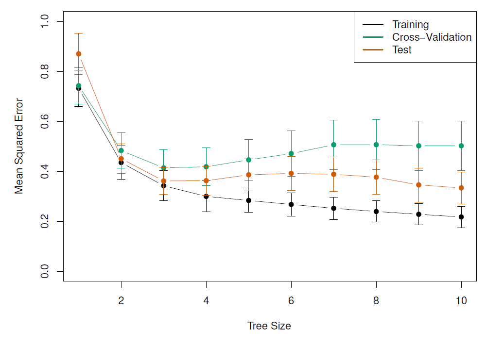
## An example: tree pruning (Hitters dataset)
- Results of fitting and pruning a regression tree on the Hitters data using 9 of the features
- Randomly divided the data set in half (132 observations in training, 131 observations in the test set)
- Built large regression tree on training data and varied $\alpha$ in Eq. 8.4 to create subtrees with different numbers of terminal nodes
- Finally, performed 6-fold cross-validation to estimate the cross-validated MSE of the trees as a function of $\alpha$
```{r}
#| label: 08-purning-a-tree
#| echo: false
#| out-width: 100%
knitr::include_graphics("images/08_5_hitters_unpruned_tree.png")
```
```{r}
#| label: 08-mse-cross-validation
#| echo: false
#| out-width: 100%
#| fig-cap: 'Training, cross-validation, and test MSE are shown as a function of the number of terminal nodes in the pruned tree. Standard error bands are displayed. The minimum cross-validation error occurs at a tree size of 3.'
knitr::include_graphics("images/08_6_hitters_mse.png")
```
## Classification trees
- Very similar to a regression tree except it predicts a qualitative (vs quantitative) response
- We predict that each observation belongs to the **most commonly occurring class** of training observations in the region to which it belongs
- In the classification setting, RSS cannot be used as a criterion for making the binary splits
- A natural alternative to RSS is the classification **error rate**, i.e., the fraction of the training observations in that region that do not belong to the most common class:
$$E = 1 - \max_k(\hat{p}_{mk})$$
where $\hat{p}_{mk}$ is the **proportion of training observations** in the $m$th region that are from the $k$th class
- However, this error rate is unsuited for tree-based classification because $E$ does not change much as the tree grows (**lacks sensitivity**)
- So, 2 other measures are preferable:
- The **Gini Index** defined by $$G = \sum_{k=1}^{K}\hat{p}_{mk}(1-\hat{p}_{mk})$$ is a measure of total variance across the K classes
- The Gini index takes on a small value if all of the $\hat{p}_{mk}$'s are close to 0 or 1
- For this reason the Gini index is referred to as a measure of node **purity** - a small value indicates that a node contains predominantly observations from a single class
- An alternative to the Gini index is **cross-entropy** given by
$$D = - \sum_{k=1}^{K}\hat{p}_{mk}\log(\hat{p}_{mk})$$
- The Gini index and cross-entropy are very similar numerically
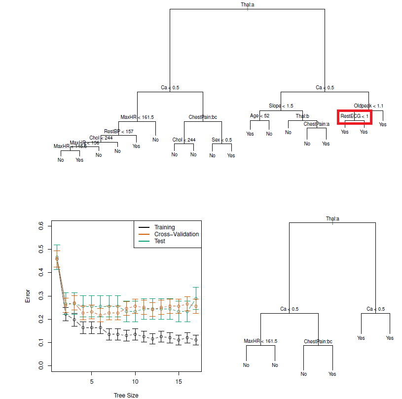
## Example: classification tree (Heart dataset)
- Data contain a binary outcome HD (heart disease Y or N based on angiographic test) for 303 patients who presented with chest pain
- 13 predictors including Age, Sex, Chol (a cholesterol measurement), and other heart and lung function measurements
- Cross-validation yields a tree with six terminal nodes
```{r}
#| label: 08-heart-dataet-cross-valudation
#| echo: false
#| out-width: 100%
#| fig-cap: 'Heart data. Top: The unpruned tree. Bottom Left: Cross-validation error, training, and test error, for different sizes of the pruned tree. Bottom Right: The pruned tree corresponding to the minimal cross-validation error.'
knitr::include_graphics("images/08_7_classif_tree_heart.png")
```
- **Comment**: Classification trees can be constructed if categorical PREDICTORS are present e.g., the first split: Thal is categorical (the 'a' in Thal:a indicates the first level of the predictor, i.e. Normal levels)
- Additionally, notice that some of the splits yield two terminal nodes that have the same predicted value (see red box)
- Regardless of the value of RestECG, a response value of *Yes* is predicted for those observations
- Why is the split performed at all?
- Because it leads to increased node purity: all 9 of the observations corresponding to the right-hand leaf have a response value of *Yes*, whereas 7/11 of those corresponding to the left-hand leaf have a response value of *Yes*
- Why is node purity important?
- Suppose that we have a test observation that belongs to the region given by that right-hand leaf. Then we can be pretty certain that its response value is *Yes*. In contrast, if a test observation belongs to the region given by the left-hand leaf, then its response value is **probably** *Yes*, but we are much less certain
- Even though the split RestECG\<1 does not reduce the classification error, it improves the Gini index and the entropy, which are more sensitive to node purity
## Advantages/Disadvantages of decision trees
- Trees can be displayed graphically and are **very easy to explain** to people
- They mirror human decision-making
- Can handle qualitative predictors without the need for dummy variables
but,
- They do not have the same level of predictive accuracy
- Can be very non-robust (i.e., a small change in the data can cause large change in the final estimated tree)
- To improve performance, we can use an **ensemble** method, which combines many simple 'buidling blocks' (i.e., regression or classification trees) to obtain a single and potentially very powerful model
- **ensemble** methods include: bagging, random forests, boosting, and Bayesian additive regression trees
## Bagging
- Also known as **bootstrap aggregation** is a general-purpose procedure for reducing the variance of a statistical learning method
- It's useful and frequently used in the context of decision trees
- Recall that given a set of $n$ independent observations $Z_1,..., Z_n$, each with variance $\sigma^2$, the variance of the mean $\bar{Z}$ of the observations is given by $\sigma^2/n$
- So, **averaging a set of observations** reduces variance
- But, this is not practical because we generally do not have access to multiple training sets!
- What can we do?
- Cue the bootstrap, i.e., take repeated samples from the single training set
- Generate $B$ different bootstrapped training data set
- Then train our method on the $b$th bootstrapped training set to get $\hat{f}^{*b}$, the prediction at a point x
- Average all the predictions to obtain $$\hat{f}_{bag}(x) = \frac{1}{B}\sum_{b=1}^B\hat{f}^{*b}(x)$$
- In the case of classification trees:
- for each test observation:
- record the class predicted by each of the $B$ trees
- take a **majority vote**: the overall prediction is the most commonly occurring class among the $B$ predictions
**Comment**: The number of trees $B$ is not a critical parameter with bagging - a large $B$ will not lead to overfitting
## Out-of-bag error estimation
- But how do we estimate the test error of a bagged model?
- It's pretty straightforward:
1. Because trees are repeatedly fit to bootstrapped subsets of observations, on average each bagged tree uses about 2/3 of the observations
2. The leftover 1/3 not used to fit a given bagged tree are called **out-of-bag** (OOB) observations
3. We can predict the response for the $i$th observation using each of the trees in which that observation was OOB. Gives around B/3 predictions for the $i$th observation (which we then average)
4. This estimate is essentially the LOO cross-validation error for bagging (if $B$ is large)
## Variable importance measures
- Bagging results in improved accuracy over prediction using a single tre
- But, it can be difficult to interpret the resulting model:
- we can't represent the statistical learning procedure using a single tree
- it's not clear which variables are most important to the procedure (i.e., we have many trees each of which may give a differing view on the importance of a given predictor)
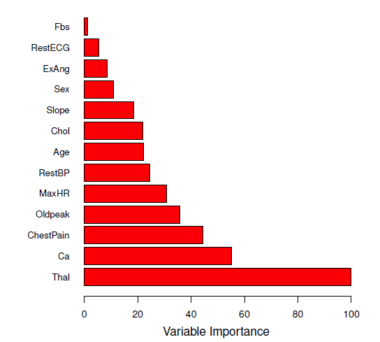
- So, which predictors are important?
- An overall summary of the importance of each predictor can be achieved by recording how much the average $RSS$ or Gini index **improves (or decreases)** when each tree is split over a given predictor (averaged over all $B$ trees)
- a large value = important predictor
```{r}
#| label: 08-variable-importance
#| echo: false
#| out-width: 100%
#| fig-cap: 'A variable importance plot for the Heart data. Variable importance is computed using the mean decrease in Gini index, and expressed relative to the maximum.'
knitr::include_graphics("images/08_8_var_importance.png")
```
## Random forests
- A problem with bagging is that bagged trees may be **highly similar** to each other.
- For example, if there is a strong predictor in the data set, most of the bagged trees will **use this strong predictor** in the top split so that
- the trees will look quite similar
- predictions from the bagged trees will be highly correlated
- Averaging many highly correlated quantities does not lead to as large a reduction in variance as averaging many uncorrelated quantities
## Random forests: advantages over bagging
- Random forests overcome this problem by forcing each split to consider only a **subset** of the predictors (typically a random sample $m \approx \sqrt{p}$)
- Thus at each split, the algorithm is NOT ALLOWED to consider a majority of the available predictors (essentially $(p - m)/p$ of the splits will not even consider the strong predictor, giving other predictors a chance)
- This *decorrelates* the trees and makes the average of the resulting trees less variable (more reliable)
- Only difference between bagging and random forests is the choice of predictor subset size $m$ at each split: if a random forest is built using $m = p$ that's just bagging
- For both, we build a number of decision trees on bootstrapped training samples
## Example: Random forests versus bagging (gene expression data)
- High-dimensional biological data set: contains gene expression measurements of 4,718 genes measured on tissue samples from 349 patients
- Each of the patient samples has a qualitative label with 15 different levels: *Normal* or one of 14 different cancer types
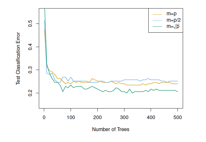
- Want to predict cancer type based on the 500 genes that have the largest variance in the training set
- Randomly divided the observations into training/test and applied random forests (or bagging) to the training set for 3 different values of $m$ (the number of predictors available at each split)
```{r}
#| label: 08-random-forest
#| echo: false
#| out-width: 100%
#| fig-cap: 'Results from random forests for the 15-class gene expression data set with p = 500 predictors. The test error is displayed as a function of the number of trees. Random forests (m < p) lead to a slight improvement over bagging (m = p). A single classification tree has an error rate of 45.7%.'
knitr::include_graphics("images/08_9_rand_forest_gene_exp.png")
```
## Boosting
- Yet another approach to improve prediction accuracy from a decision tree
- Can also be applied to many statistical learning methods for regression or classification
- Recall that in bagging each tree is built on a bootstrap training data set
- In boosting, each tree is grown sequentially using information from previously grown trees:
- given the current model, we fit a decision tree to the residuals of the model (rather than the outcome *Y*) as the response
- we then add this new decision tree into the fitted function (model) in order to update the residuals
- Why? this way each tree is built on information that the previous trees were unable to 'catch'
## Boosting algorithm
```{r}
#| label: 08-boosting-algo
#| echo: false
#| out-width: 100%
knitr::include_graphics("images/08_10_boosting_algorithm.png")
```
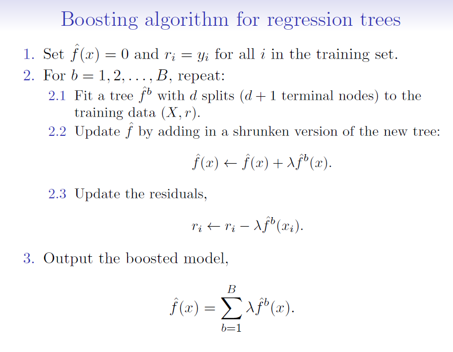
where:
$\hat{f}(x)$ is the decision tree (model)
$r$ = residuals
$d$ = number of splits in each tree (controls the complexity of the boosted ensemble)
$\lambda$ = shrinkage parameter (a small positive number that controls the rate at which boosting learns; typically 0.01 or 0.001 but right choice can depend on the problem)
- Each of the trees can be small, with just a few terminal nodes (determined by $d$)
- By fitting small trees to the residuals, we slowly improve our model ($\hat{f}$) in areas where it doesn't perform well
- The shrinkage parameter $\lambda$ slows the process down further, allowing more and different shaped trees to 'attack' the residuals
- Unlike bagging and random forests, boosting can OVERFIT if $B$ is too large. $B$ is selected via cross-validation
## Example: Boosting versus random forests
```{r}
#| label: 08-boosting-vs-rf
#| echo: false
#| out-width: 100%
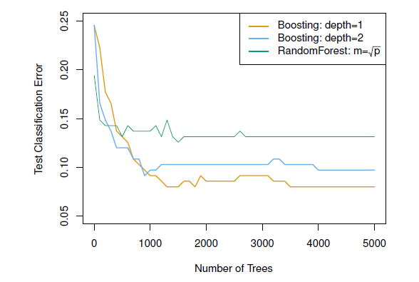
#| fig-cap: 'Results from performing boosting and random forests on the 15-class gene expression data set in order to predict cancer versus normal. The test error is displayed as a function of the number of trees. For the two boosted models, lambda = 0.01. Depth-1 trees slightly outperform depth-2 trees, and both outperform the random forest, although the standard errors are around 0.02, making none of these differences significant. The test error rate for a single tree is 24 %.'
knitr::include_graphics("images/08_11_boosting_gene_exp_data.png")
```
- Notice that because the growth of a particular tree takes into account the other trees that have already been grown, smaller trees are typically sufficient in boosting (versus random forests)
- Random forests and boosting are among the state-of-the-art methods for supervised learning (but, their results can be difficult to interpret)
## Bayesian additive regression trees (BART)
- Recall that in bagging and random forests, each tree is built on a **random sample of data and/or predictors** and each tree is built **independently** of the others
- BART is related to both - what is new is HOW the new trees are generated
- **NOTE**: only BART for regression is described in the book
## BART notation
- Let $K$ be the total **number of regression trees** and
- $B$ be the **number of iterations** the BART algorithm will run for
- Let $\hat{f}^b_k(x)$ be the **prediction** at $x$ for the $k$th regression tree used in the $b$th iteration of the BART algorithm
- At the end of each iteration, the $K$ trees from that iteration will be summed:
$$\hat{f}^b(x) = \sum_{k=1}^{K}\hat{f}^b_k(x)$$ for $b=1,...,B$
## BART algorithm
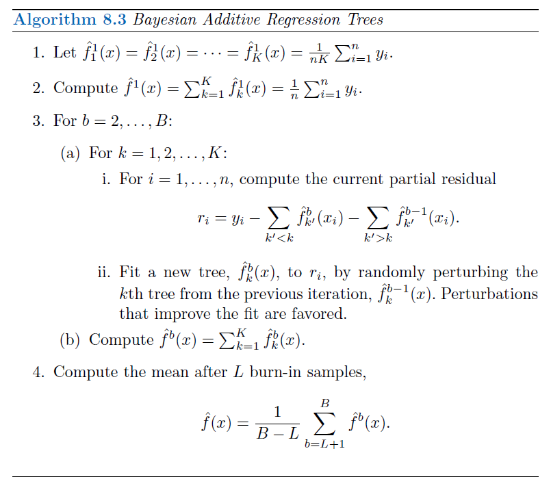
- In the first iteration of the BART algorithm, all $K$ trees are initialized to have 1 root node, with $\hat{f}^1_k(x) = \frac{1}{nK}\sum_{i=1}^{n}y_i$
- i.e., the mean of the response values divided by the total number of trees
- Thus, for the first iteration ($b = 1$), the prediction for all $K$ trees is just the mean of the response
$\hat{f}^1(x) = \sum_{k=1}^K\hat{f}^1_k(x) = \sum_{k=1}^K\frac{1}{nK}\sum_{i=1}^{n}y_i = \frac{1}{n}\sum_{i=1}^{n}y_i$
## BART algorithm: iteration 2 and on
- In subsequent iterations, BART updates each of the $K$ trees one at a time
- In the $b$th iteration to update the $k$th tree, we subtract from each response value the predictions from all but the $k$th tree, to obtain a partial residual:
$r_i = y_i - \sum_{k'<k}\hat{f}^b_{k'}(x_i) - \sum_{k'>k}\hat{f}^{b-1}_{k'}(x_i)$
for the $i$th observation, $i = 1, …, n$
- Rather than fitting a new tree to this partial residual, BART chooses a perturbation to the tree from a previous iteration $\hat{f}^{b-1}_{k}$ favoring perturbations that improve the fit to the partial residual
- To perturb trees:
- change the structure of the tree by adding/pruning branches
- change the prediction in each terminal node of the tree
- The output of BART is a collection of prediction models:
$\hat{f}^b(x) = \sum_{k=1}^{K}\hat{f}^b_k(x)$
for $b = 1, 2,…, B$
## BART algorithm: figure
```{r}
#| label: 08-bart-algo
#| echo: false
#| out-width: 100%
knitr::include_graphics("images/08_12_bart_algorithm.png")
```
- **Comment**: the first few prediction models obtained in the earlier iterations (known as the $burn-in$ period; denoted by $L$) are typically thrown away since they tend to not provide very good results, like you throw away the first pancake of the batch
## BART: additional details
- A key element of BART is that a fresh tree is NOT fit to the current partial residual: instead, we improve the fit to the current partial residual by slightly modifying the tree obtained in the previous iteration (Step 3(a)ii)
- This guards against overfitting since it limits how "hard" the data is fit in each iteration
- Additionally, the individual trees are typically pretty small
- BART, as the name suggests, can be viewed as a *Bayesian* approach to fitting an ensemble of trees:
- each time a tree is randomly perturbed to fit the residuals = drawing a new tree from a *posterior* distribution
## To apply BART:
- We must select the number of trees $K$, the number of iterations $B$ and the number of burn-in iterations $L$
- Typically, large values are chosen for $B$ and $K$ and a moderate value for $L$: e.g. $K$ = 200, $B$ = 1,000 and $L$ = 100
- BART has been shown to have impressive out-of-box performance - i.e., it performs well with minimal tuning