Applied Exercises

library(reticulate)
os <- import("os")
os$listdir(".")

 [1] "03_exercises.qmd"       ".Rhistory"              "03_main.qmd"           
 [4] "02_main.qmd"            ".Rbuildignore"          "examples.md"           
 [7] "07_exercises.qmd"       "10_exercises.qmd"       "_quarto.yml"           
[10] "bookclub-islp.Rproj"    "example_python.ipynb"   "09_main.qmd"           
[13] "08_main.qmd"            "03_video.qmd"           "06_notes.qmd"          
[16] ".DS_Store"              "12_notes.qmd"           "08_video.qmd"          
[19] "13_exercises.qmd"       "04_exercises.qmd"       "11_video.qmd"          
[22] "05_video.qmd"           "images"                 "13_main.qmd"           
[25] "12_main.qmd"            "01_notes.qmd"           "02_video.qmd"          
[28] "how-to.qmd"             "ISLP_labs_R4DS"         "example_quarto.qmd"    
[31] "13_notes.qmd"           "04_main.qmd"            "07_notes.qmd"          
[34] "05_main.qmd"            "09_video.qmd"           "06_notes.ipynb"        
[37] "docs"                   "index.qmd"              "04_video.qmd"          
[40] "09_exercises.qmd"       "10_video.qmd"           "02_notes.qmd"          
[43] "README.md"              "some_array.npy"         "08_exercises.qmd"      
[46] ".gitignore"             "figpath.png"            "01_video.qmd"          
[49] "04_notes.qmd"           ".github"                "style.css"             
[52] "10_notes.qmd"           "cover.png"              "13_video.qmd"          
[55] "07_video.qmd"           "sidebars-toggle.html"   "01_main.qmd"           
[58] "09_notes.qmd"           "03_notes.qmd"           "07_main.qmd"           
[61] "06_main.qmd"            "05_exercises.qmd"       ".git"                  
[64] "12_exercises.qmd"       "02_exercises.rmarkdown" "data"                  
[67] "11_exercises.qmd"       "06_exercises.qmd"       "_freeze"               
[70] "11_notes.qmd"           ".Rproj.user"            ".quarto"               
[73] "ISLP_data"              "05_notes.qmd"           "02_exercises.qmd"      
[76] "06_video.qmd"           "10_main.qmd"            "11_main.qmd"           
[79] "12_video.qmd"           "08_notes.qmd"


import numpy as np
import matplotlib.pyplot as plt
#%matplotlib inline
from matplotlib.pyplot import subplots
import pandas as pd
from ISLP import load_data

pd.set_option('display.max_columns', None)
#pd.set_option('display.max_rows', None)

8. This exercise relates to the `College` data set, which can be found in the file `College.csv` on the book website. It contains a number of variables for 777 different universities and colleges in the US. The variables are

Private : Public/private indicator
Apps : Number of applications received
Accept : Number of applicants accepted
Enroll : Number of new students enrolled
Top10perc : New students from top 10 % of high school class
Top25perc : New students from top 25 % of high school class
F.Undergrad : Number of full-time undergraduates
P.Undergrad : Number of part-time undergraduates
Outstate : Out-of-state tuition
Room.Board : Room and board costs
Books : Estimated book costs
Personal : Estimated personal spending
PhD : Percent of faculty with Ph.D.s
Terminal : Percent of faculty with terminal degree
S.F.Ratio : Student/faculty ratio
perc.alumni : Percent of alumni who donate
Expend : Instructional expenditure per student
Grad.Rate : Graduation rate

Before reading the data into Python, it can be viewed in Excel or a text editor.

(a) Use the `pd.read_csv()` function to read the data into `Python`. Call the loaded data `college`. Make sure that you have the directory set to the correct location for the data.

college = pd.read_csv('ISLP_data/College.csv')
college

                         Unnamed: 0 Private   Apps  Accept  Enroll  Top10perc  \
0      Abilene Christian University     Yes   1660    1232     721         23   
1                Adelphi University     Yes   2186    1924     512         16   
2                    Adrian College     Yes   1428    1097     336         22   
3               Agnes Scott College     Yes    417     349     137         60   
4         Alaska Pacific University     Yes    193     146      55         16   
..                              ...     ...    ...     ...     ...        ...   
772         Worcester State College      No   2197    1515     543          4   
773               Xavier University     Yes   1959    1805     695         24   
774  Xavier University of Louisiana     Yes   2097    1915     695         34   
775                 Yale University     Yes  10705    2453    1317         95   
776    York College of Pennsylvania     Yes   2989    1855     691         28   

     Top25perc  F.Undergrad  P.Undergrad  Outstate  Room.Board  Books  \
0           52         2885          537      7440        3300    450   
1           29         2683         1227     12280        6450    750   
2           50         1036           99     11250        3750    400   
3           89          510           63     12960        5450    450   
4           44          249          869      7560        4120    800   
..         ...          ...          ...       ...         ...    ...   
772         26         3089         2029      6797        3900    500   
773         47         2849         1107     11520        4960    600   
774         61         2793          166      6900        4200    617   
775         99         5217           83     19840        6510    630   
776         63         2988         1726      4990        3560    500   

     Personal  PhD  Terminal  S.F.Ratio  perc.alumni  Expend  Grad.Rate  
0        2200   70        78       18.1           12    7041         60  
1        1500   29        30       12.2           16   10527         56  
2        1165   53        66       12.9           30    8735         54  
3         875   92        97        7.7           37   19016         59  
4        1500   76        72       11.9            2   10922         15  
..        ...  ...       ...        ...          ...     ...        ...  
772      1200   60        60       21.0           14    4469         40  
773      1250   73        75       13.3           31    9189         83  
774       781   67        75       14.4           20    8323         49  
775      2115   96        96        5.8           49   40386         99  
776      1250   75        75       18.1           28    4509         99  

[777 rows x 19 columns]

(b) Look at the data used in the notebook by creating and running a new cell with just the code `college` in it. You should notice that the first column is just the name of each university in a column named something like `Unnamed: 0`. We don’t really want `pandas` to treat this as data. However, it may be handy to have these names for later. Try the following commands and similarly look at the resulting data frames:


college2 = pd.read_csv('ISLP_data/College.csv', index_col=0)
#college2

college3 = college.rename({'Unnamed: 0': 'college'},
  axis=1)
#college3

college3 = college3.set_index('college')
#college3

This has used the first column in the file as an index for the data frame. This means that pandas has given each row a name corresponding to the appropriate university. Now you should see that the first data column is Private. Note that the names of the colleges appear on the left of the table. We also introduced a new python object above: a dictionary, which is specified by (key, value) pairs. Keep your modified version of the data with the following:

college = college3
college

                               Private   Apps  Accept  Enroll  Top10perc  \
college                                                                    
Abilene Christian University       Yes   1660    1232     721         23   
Adelphi University                 Yes   2186    1924     512         16   
Adrian College                     Yes   1428    1097     336         22   
Agnes Scott College                Yes    417     349     137         60   
Alaska Pacific University          Yes    193     146      55         16   
...                                ...    ...     ...     ...        ...   
Worcester State College             No   2197    1515     543          4   
Xavier University                  Yes   1959    1805     695         24   
Xavier University of Louisiana     Yes   2097    1915     695         34   
Yale University                    Yes  10705    2453    1317         95   
York College of Pennsylvania       Yes   2989    1855     691         28   

                                Top25perc  F.Undergrad  P.Undergrad  Outstate  \
college                                                                         
Abilene Christian University           52         2885          537      7440   
Adelphi University                     29         2683         1227     12280   
Adrian College                         50         1036           99     11250   
Agnes Scott College                    89          510           63     12960   
Alaska Pacific University              44          249          869      7560   
...                                   ...          ...          ...       ...   
Worcester State College                26         3089         2029      6797   
Xavier University                      47         2849         1107     11520   
Xavier University of Louisiana         61         2793          166      6900   
Yale University                        99         5217           83     19840   
York College of Pennsylvania           63         2988         1726      4990   

                                Room.Board  Books  Personal  PhD  Terminal  \
college                                                                      
Abilene Christian University          3300    450      2200   70        78   
Adelphi University                    6450    750      1500   29        30   
Adrian College                        3750    400      1165   53        66   
Agnes Scott College                   5450    450       875   92        97   
Alaska Pacific University             4120    800      1500   76        72   
...                                    ...    ...       ...  ...       ...   
Worcester State College               3900    500      1200   60        60   
Xavier University                     4960    600      1250   73        75   
Xavier University of Louisiana        4200    617       781   67        75   
Yale University                       6510    630      2115   96        96   
York College of Pennsylvania          3560    500      1250   75        75   

                                S.F.Ratio  perc.alumni  Expend  Grad.Rate  
college                                                                    
Abilene Christian University         18.1           12    7041         60  
Adelphi University                   12.2           16   10527         56  
Adrian College                       12.9           30    8735         54  
Agnes Scott College                   7.7           37   19016         59  
Alaska Pacific University            11.9            2   10922         15  
...                                   ...          ...     ...        ...  
Worcester State College              21.0           14    4469         40  
Xavier University                    13.3           31    9189         83  
Xavier University of Louisiana       14.4           20    8323         49  
Yale University                       5.8           49   40386         99  
York College of Pennsylvania         18.1           28    4509         99  

[777 rows x 18 columns]

(c) Use the `describe()` method to produce a numerical summary of the variables in the data set.

college.describe()

               Apps        Accept       Enroll   Top10perc   Top25perc  \
count    777.000000    777.000000   777.000000  777.000000  777.000000   
mean    3001.638353   2018.804376   779.972973   27.558559   55.796654   
std     3870.201484   2451.113971   929.176190   17.640364   19.804778   
min       81.000000     72.000000    35.000000    1.000000    9.000000   
25%      776.000000    604.000000   242.000000   15.000000   41.000000   
50%     1558.000000   1110.000000   434.000000   23.000000   54.000000   
75%     3624.000000   2424.000000   902.000000   35.000000   69.000000   
max    48094.000000  26330.000000  6392.000000   96.000000  100.000000   

        F.Undergrad   P.Undergrad      Outstate   Room.Board        Books  \
count    777.000000    777.000000    777.000000   777.000000   777.000000   
mean    3699.907336    855.298584  10440.669241  4357.526384   549.380952   
std     4850.420531   1522.431887   4023.016484  1096.696416   165.105360   
min      139.000000      1.000000   2340.000000  1780.000000    96.000000   
25%      992.000000     95.000000   7320.000000  3597.000000   470.000000   
50%     1707.000000    353.000000   9990.000000  4200.000000   500.000000   
75%     4005.000000    967.000000  12925.000000  5050.000000   600.000000   
max    31643.000000  21836.000000  21700.000000  8124.000000  2340.000000   

          Personal         PhD    Terminal   S.F.Ratio  perc.alumni  \
count   777.000000  777.000000  777.000000  777.000000   777.000000   
mean   1340.642214   72.660232   79.702703   14.089704    22.743887   
std     677.071454   16.328155   14.722359    3.958349    12.391801   
min     250.000000    8.000000   24.000000    2.500000     0.000000   
25%     850.000000   62.000000   71.000000   11.500000    13.000000   
50%    1200.000000   75.000000   82.000000   13.600000    21.000000   
75%    1700.000000   85.000000   92.000000   16.500000    31.000000   
max    6800.000000  103.000000  100.000000   39.800000    64.000000   

             Expend  Grad.Rate  
count    777.000000  777.00000  
mean    9660.171171   65.46332  
std     5221.768440   17.17771  
min     3186.000000   10.00000  
25%     6751.000000   53.00000  
50%     8377.000000   65.00000  
75%    10830.000000   78.00000  
max    56233.000000  118.00000

(d) Use the `pd.plotting.scatter_matrix()` function to produce a scatterplot matrix of the first columns `[Top10perc, Apps, Enroll]`. Recall that you can reference a list C of columns of a data frame `A` using `A[C]`.

#fig, ax = subplots(figsize=(8, 8))
pd.plotting.scatter_matrix(college[['Top10perc','Apps','Enroll']])

array([[<AxesSubplot:xlabel='Top10perc', ylabel='Top10perc'>,
        <AxesSubplot:xlabel='Apps', ylabel='Top10perc'>,
        <AxesSubplot:xlabel='Enroll', ylabel='Top10perc'>],
       [<AxesSubplot:xlabel='Top10perc', ylabel='Apps'>,
        <AxesSubplot:xlabel='Apps', ylabel='Apps'>,
        <AxesSubplot:xlabel='Enroll', ylabel='Apps'>],
       [<AxesSubplot:xlabel='Top10perc', ylabel='Enroll'>,
        <AxesSubplot:xlabel='Apps', ylabel='Enroll'>,
        <AxesSubplot:xlabel='Enroll', ylabel='Enroll'>]], dtype=object)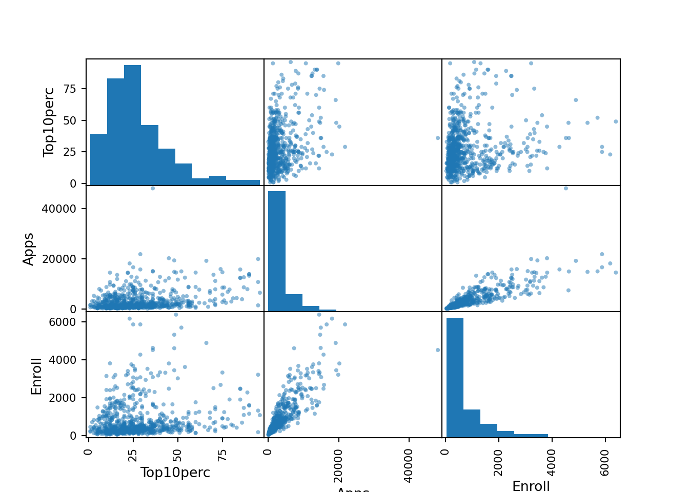

#plt.show()

(e) Use the boxplot() method of college to produce side-by-side boxplots of Outstate versus Private.

(f) Create a new qualitative variable, called Elite, by binning the Top10perc variable into two groups based on whether or not the proportion of students coming from the top 10% of their high school classes exceeds 50%.

college['Elite'] = pd.cut(college['Top10perc'],
  [0,0.5,1],
  labels=['No', 'Yes'])

Use the value_counts() method of college['Elite'] to see how many elite universities there are. Finally, use the boxplot() method again to produce side-by-side boxplots of Outstate versus Elite.

college['Elite'].value_counts()

Yes    3
No     0
Name: Elite, dtype: int64

(g) Use the `plot.hist()` method of `college` to produce some histograms with difering numbers of bins for a few of the quantitative variables. The command `plt.subplots(2, 2)` may be useful: it will divide the plot window into four regions so that four plots can be made simultaneously. By changing the arguments you can divide the screen up in other combinations.

(h) Continue exploring the data, and provide a brief summary of what you discover.

9. This exercise involves the `Auto` data set studied in the lab. Make sure that the missing values have been removed from the data.

Auto = pd.read_csv('ISLP_data/Auto.csv',
                    na_values=['?'])
Auto

      mpg  cylinders  displacement  horsepower  weight  acceleration  year  \
0    18.0          8         307.0       130.0    3504          12.0    70   
1    15.0          8         350.0       165.0    3693          11.5    70   
2    18.0          8         318.0       150.0    3436          11.0    70   
3    16.0          8         304.0       150.0    3433          12.0    70   
4    17.0          8         302.0       140.0    3449          10.5    70   
..    ...        ...           ...         ...     ...           ...   ...   
392  27.0          4         140.0        86.0    2790          15.6    82   
393  44.0          4          97.0        52.0    2130          24.6    82   
394  32.0          4         135.0        84.0    2295          11.6    82   
395  28.0          4         120.0        79.0    2625          18.6    82   
396  31.0          4         119.0        82.0    2720          19.4    82   

     origin                       name  
0         1  chevrolet chevelle malibu  
1         1          buick skylark 320  
2         1         plymouth satellite  
3         1              amc rebel sst  
4         1                ford torino  
..      ...                        ...  
392       1            ford mustang gl  
393       2                  vw pickup  
394       1              dodge rampage  
395       1                ford ranger  
396       1                 chevy s-10  

[397 rows x 9 columns]

(a) Which of the predictors are quantitative, and which are qualitative?

Mpg, Displacement, Horsepower, Weight and Acceleration are quantitative. Cylinders, Year, Origin, and Name are qualitative.

Auto.info()

<class 'pandas.core.frame.DataFrame'>
RangeIndex: 397 entries, 0 to 396
Data columns (total 9 columns):
 #   Column        Non-Null Count  Dtype  
---  ------        --------------  -----  
 0   mpg           397 non-null    float64
 1   cylinders     397 non-null    int64  
 2   displacement  397 non-null    float64
 3   horsepower    392 non-null    float64
 4   weight        397 non-null    int64  
 5   acceleration  397 non-null    float64
 6   year          397 non-null    int64  
 7   origin        397 non-null    int64  
 8   name          397 non-null    object 
dtypes: float64(4), int64(4), object(1)
memory usage: 28.0+ KB

Auto['cylinders'] = Auto['cylinders'].astype('object') 
Auto['cylinders']

0      8
1      8
2      8
3      8
4      8
      ..
392    4
393    4
394    4
395    4
396    4
Name: cylinders, Length: 397, dtype: object

(b) What is the range of each quantitative predictor? You can answer this using the `min()` and `max()` methods in `numpy`.

mpg_min = Auto['mpg'].min( )
mpg_max = Auto['mpg'].max( )

print('The min and max miles per gallon are', (mpg_min, mpg_max))

The min and max miles per gallon are (9.0, 46.6)

dsp_min = Auto['displacement'].min( )
dsp_max = Auto['displacement'].max( )

print('The min and max displacement are', (dsp_min, dsp_max))

The min and max displacement are (68.0, 455.0)

hpwr_min = Auto['horsepower'].min( )
hpwr_max = Auto['horsepower'].max( )

print('The min and max horsepower are', (hpwr_min, hpwr_max))

The min and max horsepower are (46.0, 230.0)

wt_min = Auto['weight'].min( )
wt_max = Auto['weight'].max( )

print('The min and max weights are', (wt_min, wt_max))

The min and max weights are (1613, 5140)

acc_min = Auto['acceleration'].min( )
acc_max = Auto['acceleration'].max( )

print('The min and max accelerations are', (acc_min, acc_max))

The min and max accelerations are (8.0, 24.8)

(c) What is the mean and standard deviation of each quantitative predictor?

mpg_mean = Auto['mpg'].mean( )
mpg_sd = Auto['mpg'].std( )

print('The mean and standard deviation of miles per gallon are', mpg_mean,'and', mpg_sd)

The mean and standard deviation of miles per gallon are 23.515869017632248 and 7.825803928946562

dsp_mean = Auto['displacement'].mean( )
dsp_sd = Auto['displacement'].std( )

print('The mean and standard deviation of weight are', dsp_mean,'and', dsp_sd)

The mean and standard deviation of weight are 193.53274559193954 and 104.37958329992945

hpwr_mean = Auto['horsepower'].mean( )
hpwr_sd = Auto['horsepower'].std( )

print('The mean and standard deviation of horsepower are', hpwr_mean,'and', hpwr_sd)

The mean and standard deviation of horsepower are 104.46938775510205 and 38.49115993282855

wt_mean = Auto['weight'].mean( )
wt_sd = Auto['weight'].std( )

print('The mean and standard deviation of weight are', wt_mean,'and', wt_sd)

The mean and standard deviation of weight are 2970.2619647355164 and 847.9041194897246

acc_mean = Auto['acceleration'].mean( )
acc_sd = Auto['acceleration'].std( )

print('The mean and standard deviation of acceleration are', acc_mean,'and', acc_sd)

The mean and standard deviation of acceleration are 15.555667506297214 and 2.7499952929761515

(d) Now remove the 10th through 85th observations. What is the range, mean, and standard deviation of each predictor in the subset of the data that remains?

Auto_new = Auto.drop(Auto.index[10:85])
Auto_new

      mpg cylinders  displacement  horsepower  weight  acceleration  year  \
0    18.0         8         307.0       130.0    3504          12.0    70   
1    15.0         8         350.0       165.0    3693          11.5    70   
2    18.0         8         318.0       150.0    3436          11.0    70   
3    16.0         8         304.0       150.0    3433          12.0    70   
4    17.0         8         302.0       140.0    3449          10.5    70   
..    ...       ...           ...         ...     ...           ...   ...   
392  27.0         4         140.0        86.0    2790          15.6    82   
393  44.0         4          97.0        52.0    2130          24.6    82   
394  32.0         4         135.0        84.0    2295          11.6    82   
395  28.0         4         120.0        79.0    2625          18.6    82   
396  31.0         4         119.0        82.0    2720          19.4    82   

     origin                       name  
0         1  chevrolet chevelle malibu  
1         1          buick skylark 320  
2         1         plymouth satellite  
3         1              amc rebel sst  
4         1                ford torino  
..      ...                        ...  
392       1            ford mustang gl  
393       2                  vw pickup  
394       1              dodge rampage  
395       1                ford ranger  
396       1                 chevy s-10  

[322 rows x 9 columns]

mpg_min = Auto_new['mpg'].min( )
mpg_max = Auto_new['mpg'].max( )

print('The min and max miles per gallon of the subsetted data are', (mpg_min, mpg_max))

The min and max miles per gallon of the subsetted data are (11.0, 46.6)

mpg_mean = Auto_new['mpg'].mean( )
mpg_sd = Auto_new['mpg'].std( )

print('The mean and standard deviation of miles per gallon of the subsetted data are', mpg_mean,'and', mpg_sd)

The mean and standard deviation of miles per gallon of the subsetted data are 24.40931677018633 and 7.913357147165568

dsp_min = Auto_new['displacement'].min( )
dsp_max = Auto_new['displacement'].max( )

print('The min and max displacement of the subsetted data are', (dsp_min, dsp_max))

The min and max displacement of the subsetted data are (68.0, 455.0)

dsp_mean = Auto_new['displacement'].mean( )
dsp_sd = Auto_new['displacement'].std( )

print('The mean and standard deviation of weight of the subsetted data are', dsp_mean,'and', dsp_sd)

The mean and standard deviation of weight of the subsetted data are 187.6801242236025 and 100.12092459330134

hpwr_min = Auto['horsepower'].min( )
hpwr_max = Auto['horsepower'].max( )

print('The min and max horsepower of the subsetted data are', (hpwr_min, hpwr_max))

The min and max horsepower of the subsetted data are (46.0, 230.0)

hpwr_mean = Auto['horsepower'].mean( )
hpwr_sd = Auto['horsepower'].std( )

print('The mean and standard deviation of horsepower of the subsetted data are', hpwr_mean,'and', hpwr_sd)

The mean and standard deviation of horsepower of the subsetted data are 104.46938775510205 and 38.49115993282855

wt_min = Auto['weight'].min( )
wt_max = Auto['weight'].max( )

print('The min and max weights of the subsetted data are', (wt_min, wt_max))

The min and max weights of the subsetted data are (1613, 5140)

wt_mean = Auto['weight'].mean( )
wt_sd = Auto['weight'].std( )

print('The mean and standard deviation of weight of the subsetted data are', wt_mean,'and', wt_sd)

The mean and standard deviation of weight of the subsetted data are 2970.2619647355164 and 847.9041194897246

acc_min = Auto['acceleration'].min( )
acc_max = Auto['acceleration'].max( )

print('The min and max accelerations of the subsetted data are', (acc_min, acc_max))

The min and max accelerations of the subsetted data are (8.0, 24.8)

acc_mean = Auto['acceleration'].mean( )
acc_sd = Auto['acceleration'].std( )

print('The mean and standard deviation of acceleration of the subsetted data are', acc_mean,'and', acc_sd)

The mean and standard deviation of acceleration of the subsetted data are 15.555667506297214 and 2.7499952929761515

(e) Using the full data set, investigate the predictors graphically, using scatterplots or other tools of your choice. Create some plots highlighting the relationships among the predictors. Comment on your findings.

(f) Suppose that we wish to predict gas mileage (`mpg`) on the basis of the other variables. Do your plots suggest that any of the other variables might be useful in predicting `mpg`? Justify your answer.

10. This exercise involves the `Boston` housing data set.

(a) To begin, load in the `Boston` data set, which is part of the `ISLP` library.

Boston = load_data("Boston")
Boston

        crim    zn  indus  chas    nox     rm   age     dis  rad  tax  \
0    0.00632  18.0   2.31     0  0.538  6.575  65.2  4.0900    1  296   
1    0.02731   0.0   7.07     0  0.469  6.421  78.9  4.9671    2  242   
2    0.02729   0.0   7.07     0  0.469  7.185  61.1  4.9671    2  242   
3    0.03237   0.0   2.18     0  0.458  6.998  45.8  6.0622    3  222   
4    0.06905   0.0   2.18     0  0.458  7.147  54.2  6.0622    3  222   
..       ...   ...    ...   ...    ...    ...   ...     ...  ...  ...   
501  0.06263   0.0  11.93     0  0.573  6.593  69.1  2.4786    1  273   
502  0.04527   0.0  11.93     0  0.573  6.120  76.7  2.2875    1  273   
503  0.06076   0.0  11.93     0  0.573  6.976  91.0  2.1675    1  273   
504  0.10959   0.0  11.93     0  0.573  6.794  89.3  2.3889    1  273   
505  0.04741   0.0  11.93     0  0.573  6.030  80.8  2.5050    1  273   

     ptratio  lstat  medv  
0       15.3   4.98  24.0  
1       17.8   9.14  21.6  
2       17.8   4.03  34.7  
3       18.7   2.94  33.4  
4       18.7   5.33  36.2  
..       ...    ...   ...  
501     21.0   9.67  22.4  
502     21.0   9.08  20.6  
503     21.0   5.64  23.9  
504     21.0   6.48  22.0  
505     21.0   7.88  11.9  

[506 rows x 13 columns]

(b) How many rows are in this data set? How many columns? What do the rows and columns represent?

(c) Make some pairwise scatterplots of the predictors (columns) in this data set. Describe your fndings.

(d) Are any of the predictors associated with per capita crime rate? If so, explain the relationship.

(e) Do any of the suburbs of Boston appear to have particularly high crime rates? Tax rates? Pupil-teacher ratios? Comment on the range of each predictor.

(f) How many of the suburbs in this data set bound the Charles river?

(g) What is the median pupil-teacher ratio among the towns in this data set?

(h) Which suburb of Boston has lowest median value of owneroccupied homes? What are the values of the other predictors for that suburb, and how do those values compare to the overall ranges for those predictors? Comment on your fndings.

(i) In this data set, how many of the suburbs average more than seven rooms per dwelling? More than eight rooms per dwelling? Comment on the suburbs that average more than eight rooms per dwelling.

8. This exercise relates to the College data set, which can be found in the file College.csv on the book website. It contains a number of variables for 777 different universities and colleges in the US. The variables are

(a) Use the pd.read_csv() function to read the data into Python. Call the loaded data college. Make sure that you have the directory set to the correct location for the data.

(c) Use the describe() method to produce a numerical summary of the variables in the data set.

(d) Use the pd.plotting.scatter_matrix() function to produce a scatterplot matrix of the first columns [Top10perc, Apps, Enroll]. Recall that you can reference a list C of columns of a data frame A using A[C].