17. Scaling Laws
2025-04-13
Chapter 17: Scaling Laws
Goal: Understand how scale predicts LLM performance
Builds on: Pretraining, Distributed Training
We’ll cover:
What are scaling laws?
Power laws: the foundation
Scaling laws in deep learning
The Chinchilla scaling law Implications and limitations
The “bitter lesson” of AI research
What Are Scaling Laws?
- Scaling Laws describe how changes in model size, dataset size, or compute affect AI model performance.
- They are essential for understanding and optimizing AI models.
- Predict how LLM performance (loss) changes with:
- Model size (parameters)
- Dataset size (tokens)
- Compute (FLOPs)
- Allow us to make reliable predictions about model performance
- Enable optimization of hyperparameters without expensive grid searches
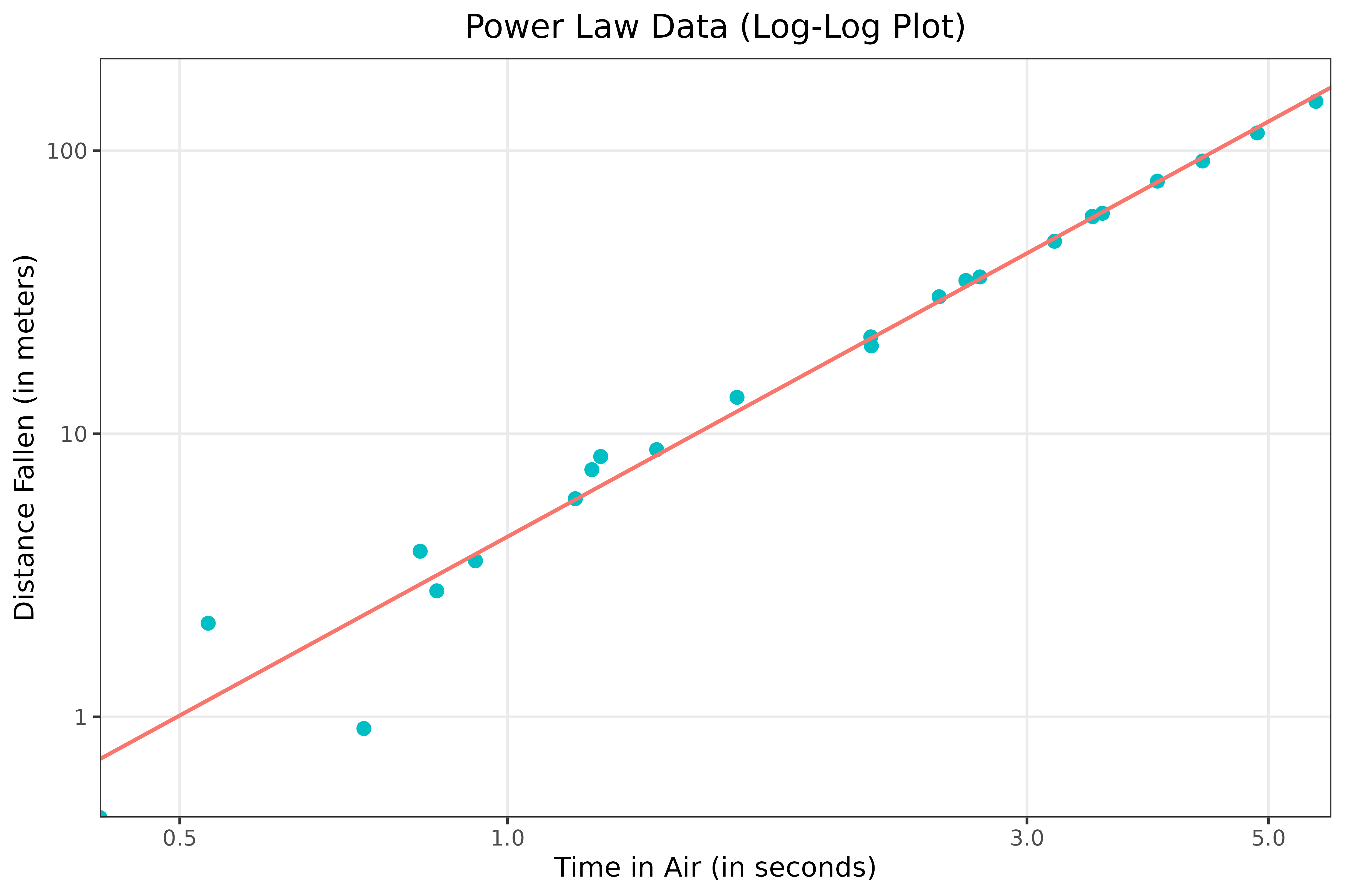
Power Laws: The Foundation
Power laws: mathematical equations of the form: y = bx^a
Describe how one quantity varies as the power of another
- y : Performance (e.g., loss), x : Scale (e.g., parameters)
On a log-log plot, Power laws = straight lines
![]()
Scaling Laws in Deep Learning: why scaling laws matter
- In deep learning, performance scales according to:
- N: Model size (number of parameters)
- D: Dataset size (tokens, pixels, etc.)
- C: Compute (FLOPs)
- As these variables increase, model loss decreases following power laws
- Scaling is primarily bottlenecked by computational resources
Key Variables in Scaling Laws
Model Size (N):
Number of parameters (weights) in the model
Measures model capacity
Dataset Size (D):
Number of tokens the model is trained on
Tokens can be words, subwords, pixels, etc.
Compute (C):
Floating point operations (FLOPs) used during training
Enables both larger models and more training data
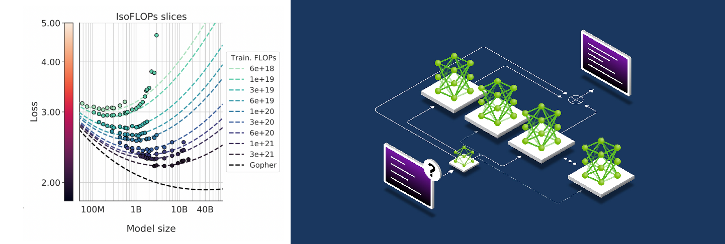
The Chinchilla Scaling Law
- Key paper (Hoffmann et al. 2022): “Training Compute-Optimal LLMs”
- Finding: Balance model size & data for compute budget
- Introduced by Hoffmann et al. (2022)
- Key insight: optimal performance requires balancing model and data size
Small models with more training data can outperform larger models
Chinchilla (70B params) beat larger models with more tokens
Chinchilla in Action
Implications
- Planning: Predict performance before training
- Efficiency: Avoid oversized models
- Cost: Optimize compute allocation
- Ties to distributed training’s scale (Ch. 16)
Universal Applicability
- Scaling laws hold across many modalities and orders of magnitude.
- Generative models (e.g., LLMs) follow scaling laws.
- Strong for generative models (e.g., LLMs)
- Weaker for discriminative models (e.g., image classifiers)
- Algorithms can shift the curve (better constant terms)
The Bitter Lesson
Key observation: Scaling beats intricate, expert-designed systems.
Simpler systems trained on more data outperform complex, human-designed approaches.
Lesson: Invest in compute and data rather than manual feature engineering.
Scaling often beats complex designs
Challenges & Debates
- Chinchilla’s exact numbers contested
- Scaling laws are not universal.
- Equations are debated and subject to refinement.
- Future trends: Scaling laws may evolve as models and tasks become more complex.
- Replication issues (see Eleuther AI post)
- Future laws may refine predictions
Implications for AI Development
Resource allocation: Optimize the ratio of model size to dataset size
Investment focus: Compute is the fundamental bottleneck
Research priorities: Algorithm improvements can shift the scaling curve
Future capabilities: May be predictable through extrapolation
AI timelines: Scaling laws inform predictions about AI progress
Key Takeaways
- Scaling laws predict loss via params, data, compute
- Chinchilla: Balance scale for efficiency
- Power laws = reliable trends, but not universal
- Optimize training smarter, not harder
Resources
- “Chinchilla Scaling Laws” by Rania Hossam
- “Chinchilla’s Wild Implications” (LessWrong)
- “Scaling Laws and Emergent Properties” by Clément Thiriet
- Stanford CS224n “Scaling Language Models” video
Q&A
True or False: Scaling laws apply to all ML models
False. Generative models (e.g., LLMs) follow clear scaling laws, but discriminative models (e.g., image classifiers) often don’t.
How does compute relate to scaling?
Compute drives scaling by enabling larger models and datasets. More FLOPs = more parameters or tokens.
What’s a power law?
A power law is ( y = bx^a ), where ( y ) (e.g., loss) scales with ( x ) (e.g., params) raised to an exponent. It’s linear on a log-log plot.