Generative AI Handbook Book Club – 15. Pretraining Recipes

What is Pretraining?

Training an LLM from scratch on a large corpus (e.g., Common Crawl)
Objective: Predict next token in text
Output: A “base” model for later finetuning
Connects to decoder-only Transformers (Section II)

Pretraining: The Big Picture

Process of training a model on vast amounts of text data
Self-supervised learning: predict next token or masked tokens
Goal: Develop general language understanding capabilities
Resource-intensive: requires significant compute, data, engineering
Many design choices affect training efficiency and model quality

Building on Previous Chapters

Transformer Architecture: Foundation of modern LLMs
Tokenization: Converting text to model-readable tokens
Positional Encoding: Representing sequence information
Here we examine: How to effectively train these models?

Core Architectural Choices

Key decisions when pretraining LLMs:

Attention mechanisms
Activation functions
Normalization approaches
Model sizing & dimensionality

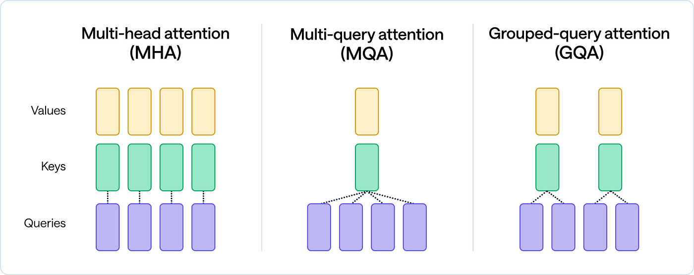
Attention Mechanism Variants

Three main approaches:

Multi-Head Attention (MHA): - Original Transformer design - Multiple attention heads, each with full query/key/value projections - Most expressive but computationally expensive
Multi-Query Attention (MQA): - Shared key and value projections across heads - Queries remain separate - Reduces memory bandwidth requirements
Grouped-Query Attention (GQA): - Middle ground between MHA and MQA - Keys and values shared among groups of heads - Better balance of efficiency and expressiveness

Key Decisions in Pretraining

No one-size-fits-all “recipe”
Choices impact performance, cost, speed
Core areas:
- Model architecture (e.g., attention)
- Training setup (e.g., optimization)
- Data handling

Attention Variants: Trade-offs

Variant	Parameters	Memory	Quality	Used In
MHA	Highest	Highest	Highest	Early models, high-quality research
MQA	Lowest	Lowest	Lowest	Deployment-optimized models
GQA	Medium	Medium	Medium	Modern balanced models (Claude, PaLM)

Attention Variants: MQA vs GQA vs MHA

Attention Variants Comparison

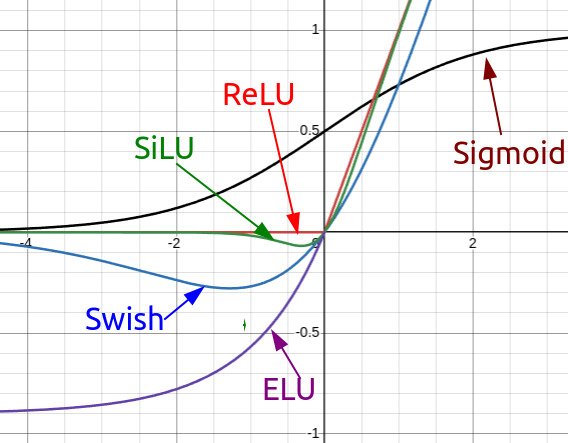
Activation Functions

Evolution of activation functions in LLMs:

- ReLU: Simple, efficient, but limited expressiveness
- GeLU: Smoother variant of ReLU, used in many models
- SwiGLU: Swish + GLU combination, better performance - Used in PaLM, LLaMA, and other recent models - Computationally more expensive but better results

Impacts how neurons “fire” in Transformers

Plot of ReLU vs. GeLU

SwiGLU: The Modern Standard

SwiGLU computation:

$\text{SwiGLU}(x) = \text{Swish}(xW) \otimes (xV)$

Where:

$\text{Swish}(x) = x \cdot \text{sigmoid}(\beta x)$
$\otimes \text{ denotes element-wise multiplication}$

Benefits:

Better gradient flow
Improved representational capacity
Modest compute overhead for significant quality gains

Normalization Techniques

Layer Normalization: Standard in Transformers
- Normalizes across feature dimension
- Stabilizes training
RMSNorm: Simplified version of LayerNorm
- Removes mean-centering step
- Slightly faster computation
- Used in LLaMA and other recent models

Optimization Strategies

Key components:

Optimizer choice
Learning rate scheduling
Weight decay
Gradient clipping

Optimizers for LLMs

AdamW: Standard choice for most LLMs
- Adaptive learning rates with proper weight decay
- Robust to hyperparameter choices
Adafactor: Memory-efficient alternative
- Factorizes second moment matrices
- Useful for memory-constrained settings
Lion: Recent lightweight optimizer
- Momentum-based with sign updates
- Less memory usage, competitive performance

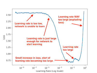
Learning Rate Scheduling

Typical LLM learning rate schedule:

Warmup phase: Gradually increase from small value
- Prevents early instability
- Usually 1-3% of total training steps
Decay phase: Gradual reduction of learning rate
- Cosine decay: Smooth reduction to minimum value
- Linear decay: Simpler alternative

Learning Rate Schedule

Effective Batch Sizing

Global batch size: Total number of sequences processed before update
Micro-batch size: Sequences processed on each device
Gradient accumulation: Accumulate gradients over multiple micro-batches

Key considerations: - Larger batches → better gradient estimates but diminishing returns - Memory constraints often limit micro-batch size - Typical global batch sizes: 1-8 million tokens

Dropout Strategies

Early LLMs: Significant dropout (0.1-0.2)
Modern trend: Minimal or no dropout
- Chinchilla scaling laws: data > regularization
- Current practice: Use dropout only for small models or limited data
When used, applied to:
- Attention outputs
- Feed-forward outputs
- Embedding layers

Training Duration and Data Reuse

Epoch: One pass through the entire dataset
Modern LLMs rarely see full epochs
Tokens seen during training:
- GPT-3: 300B tokens
- PaLM: 780B tokens
- LLaMA 2: 2T tokens
- Claude/GPT-4: 10T+ tokens (estimated)
Data mixing: Different sources with different sampling weights
Data repetition: Strategic repeating of high-quality data

Scaling Laws and Compute-Optimal Training

Chinchilla scaling laws (DeepMind, 2022):
- Model size and training data should scale together
- Optimal tokens ≈ 20x parameter count
- E.g., 70B model → 1.4T tokens for optimal training
Compute-optimal training:
- Balance model size, data, and training time given fixed compute budget

Hyperparameter Selection

Modern approach: Much less tuning than traditional ML
Focus on proven defaults from literature
Key hyperparameters to tune:
- Learning rate and schedule
- Weight decay
- Model width/depth ratio
- Global batch size

Engineering Considerations

Mixed precision training: fp16/bf16 + fp32 optimizer states
Gradient checkpointing: Trade computation for memory
Model parallelism: Distribute model across devices
Data parallelism: Process different batches on different devices
Zero Redundancy Optimizer (ZeRO): Partition optimizer states
FlashAttention: Efficient attention implementation

Industry Best Practices

Recent trends from leading labs:

GQA + SwiGLU + RMSNorm architecture
AdamW optimizer with cosine decay
2-4M token batch sizes
Minimal dropout
Compute-optimal training allocation
Heavy use of data curation and filtering

Resources

A Recipe for Training Neural Networks by Andrej Karpathy
The Novice’s LLM Training Guide by Alpin Dale
Navigating the Attention Landscape by Shobhit Agarwal
Chinchilla scaling laws paper

Key Takeaways

Many architectural and training choices affect LLM performance
Modern defaults have emerged through industry experimentation
Balancing compute efficiency and model quality is crucial
Both architecture and optimization strategy matter significantly
No single “best recipe” - depends on resources and goals