Generative AI Handbook Book Club – 5. Reinforcement Learning

Textbook

Markov Decision Process

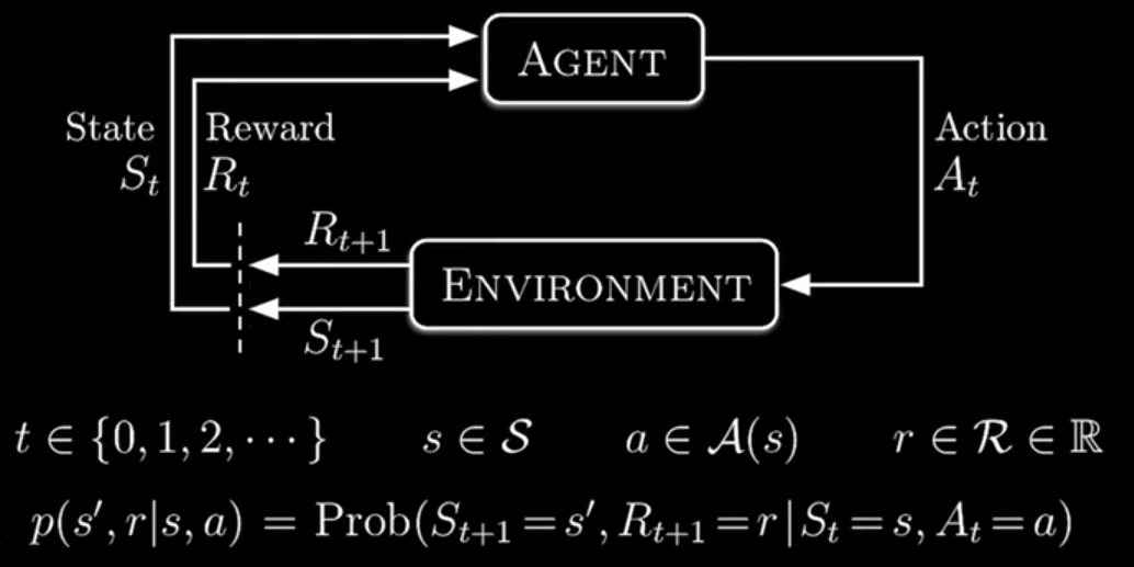
MDP

Objective

policy: $\pi(a|s)$
return: $G_{t} = \sum_{k=t+1}^{T} \gamma^{k-t-1}R_{k}$
maximize expected return over all policies

$\text{max}_{\pi} \text{E}_{\pi}[G_{t}]$

Coupled Equations

state value function

$v_{\pi}(s) = \text{E}_{\pi}[G_{t}|S_{t} = s]$

action value function

$q_{\pi}(s,a) = \text{E}_{\pi}[G_{t}|S_{t} = s, A_{t} = a]$

Bellman Equations

connect all state values

$\begin{array}{rcl} v_{\pi}(s^{i}) & = & \text{E}_{\pi}[G_{t}|s^{i}] \\ ~ & = & \sum_{\{a\}} \pi(a|s^{i}) \cdot q(s^{i},a) \\ ~ & = & \sum_{\{a\}} \pi(a|s^{i}) \cdot \text{E}_{\pi}[G_{t}|s^{i}, a] \\ \end{array}$

Bellman Optimality Equations

For any optimal $\pi_{*}$ , $\forall s \in S$ , $\forall a \in A$

$\begin{array}{rcl} v_{*}(s) & = & \text{max}_{a} q_{*}(s,a) \\ q_{*}(s,a) & = & \sum_{s,r} p(s'r|s,a)[r + \gamma v_{*}(s')] \\ \end{array}$

Monte Carlo Methods

We do not know $p(s'r|s,a)$

generate samples: $S_{0}, A_{0}, R_{1}, S_{1}, A_{1}, R_{2}, ...$
obtain averages $\approx$ expected values
generalized policy iteration to obtain

$\pi \approx \pi_{*}$

Monte Carlo Evaluation

approx $v_{\pi}(s)$

$\text{E}_{\pi}[G_{t}|S_{t} = s] \approx \frac{1}{C(s)}\sum_{m=1}^{M}\sum_{\tau=0}^{T_{m}-1} I(s_{\tau}^{m} = s)g_{\tau}^{m}$ * step size $\alpha$ for update rule

$V(s_{t}^{m}) \leftarrow V(s_{t}^{m}) + \alpha\left(g_{t}^{m} - V(s_{t}^{m})\right)$

Exploration-Exploitation Trade-Off

to discover optimal policies

we must explroe all state-action pairs

to get high returns

we must exploit known high-value pairs

Example: Blackjack

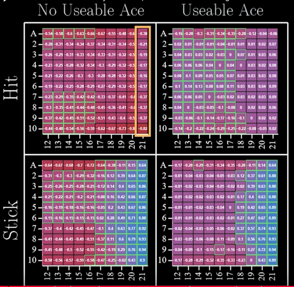
MCMC solving blackjack game

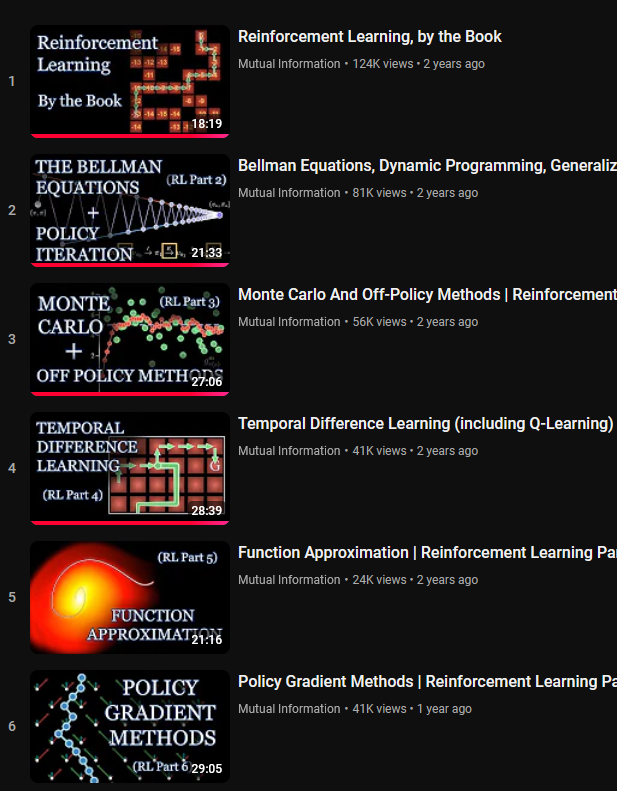
image credit: Mutual Information

10 million games played

Temporal Difference Learning

Markov Reward Process: A Markov decision process, but w/o actions
MCMC requires an episode to complete before updating

but what if an episode is long?

n-step TD

Replace $g_{t}^{m}$ with

$g_{t:t+n}^{m} = r_{t+1}^{m} + \gamma r_{t+2}^{m} + \cdots + \gamma^{n-1} r_{t+n}^{m} + \gamma_{n}V(s_{t+n}^{m})$

updates are applied during the episoes with an n-step delay

Advantages

Compared to MC, TD has

batch training
$V(s)$ do not depend on stepsize $\alpha$
max likelihood of MRP (instead of min MSE)

Q-Learning

$r_{t+1}^{m} + \gamma \text{max}_{a} Q(s_{t+1}^{m},a)$

updates $Q$ after each sarsa tuple (each n-step delay)

Toward Continuity

previous methods assumed tabular (discrete) and finite state spaces
without “infinite data”, can we still generalize?
function approximation: supervised learning + reinforcement learning

Parameter Space

$v_{\pi}(s) \approx \hat{v}(s,w), \quad w \in \mathbb{R}^{d}$ * caution: updating $w$ updates many values of $s$

not just the “visited states”

Value Error

$\text{VE}(w) = \sum_{s \in S} \mu(s)\left[v_{\pi}(s) - \hat{v}(s,w)\right]^{2}$

$\mu$ : distribution of states
solve with stochastic gradient descent

$w \leftarrow w + \alpha\left[U_{t} - \hat{v}(S_{t},w)\right] \nabla \hat{v}(S_{t},w)$

Target Selection

To find target $U_{t}$

may have multiple local minima
estimates for state values may be biased
employ Semi-Gradient Temporal Difference