Rewriting R code in C++ (and Rust)
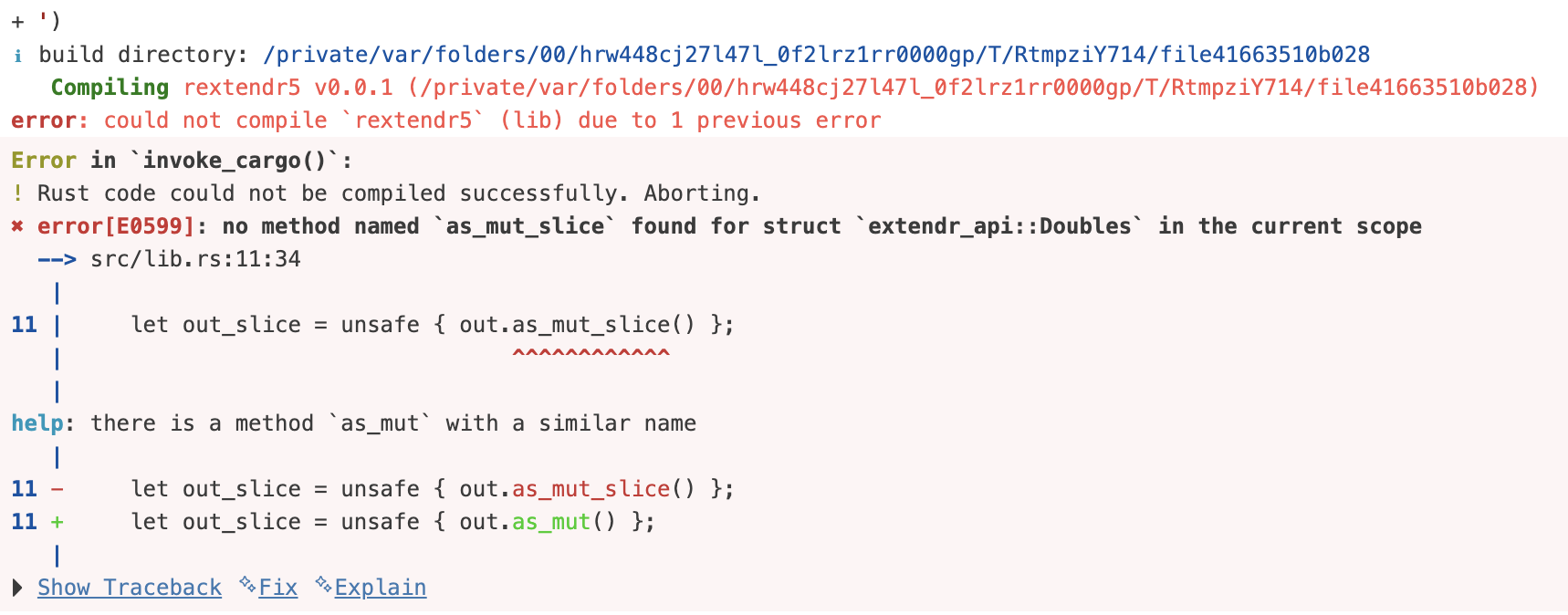
Rust has more readable error messages than C++
#> using C++ compiler: ‘g++ (Ubuntu 13.3.0-6ubuntu2~24.04) 13.3.0’
#> g++ -std=gnu++17 -I"/opt/R/4.5.2/lib/R/include" -DNDEBUG   -I"/home/runner/work/_temp/Library/Rcpp/include" -I"/tmp/RtmpqdbWeh/sourceCpp-x86_64-pc-linux-gnu-1.1.1" -I/usr/local/include    -fpic  -g -O2   -c file1de4260813f2.cpp -o file1de4260813f2.o
#> file1de4260813f2.cpp: In function ‘Rcpp::NumericVector signCfaster(Rcpp::NumericVector)’:
#> file1de4260813f2.cpp:12:15: error: ‘v’ was not declared in this scope
#>    12 |     out[i] = (v > 0) ? 1.0 : (v == 0 ? 0.0 : -1.0);
#>       |               ^
#> make: *** [/opt/R/4.5.2/lib/R/etc/Makeconf:211: file1de4260813f2.o] Error 1
#> Error in `sourceCpp()`:
#> ! Error 1 occurred building shared library.rextendr::rust_function('
fn signRustSlice(x: Robj) -> Robj {
// Borrow numeric slice from R (no copy)
let slice = x.as_real_slice().expect("Expected numeric vector");
let n = slice.len();
let mut out = Doubles::new(n);
// Unsafe block gives direct mutable slice (no bounds checks)
let out_slice = unsafe { out.as_mut_slice() };
for i in 0..n {
let v = slice[i];
out_slice[i] = if v.is_nan() {
f64::NAN
} else if v > 0.0 {
1.0
} else if v == 0.0 {
0.0
} else {
-1.0
};
}
out.into()
}
')