Translating R code
Learning objectives:
- Understand what it means to translate R code
- Treat code as data to enable domain-specific languages (DSLs)
- Create HTML and LaTeX DSLs
- Learn how environments, S3, and metaprogramming work together
What does translating R code mean?
R code → another language
Translating code is not the same as evaluating code
- Evaluation produces a value (
3) - Translation preserves structure (
sqrt(x)) - The result is code, not a computed number
Code translation relies on metaprogramming
- Expressions are captured with
expr()/enexpr() - Calls, symbols, etc… can be inspected
- Translation operates on the AST, not on values
The practical goal of translation is domain-specific languages
- DSLs embed a small language inside R
- R syntax becomes a frontend for another language
dbplyras an example: R → SQL
Fundamentals of R → HTML
We can generate HTML code from R
- We can do this…
- By doing this…
Basically, HTML tags become “ordinary” R functions
Our DSL makes translation easy
Same structure: nesting of function calls == nesting of tags.
Similar logic: unnamed arguments -> tag content, named arguments -> tag attributes.
User experience: special characters automatically escaped (e.g.
"&"->"&").
We need five basic HTML tags for this exercise
<body>is the top-level tag that contains all content.<h1>defines a top level heading.<p>defines a paragraph.<b>emboldens text.<img>embeds an image.
We need to know the main structure of tags
- Main tags structure:
<tag> </tag> - Void tags structure:
<tag /> - Tags can have attributes:
<tag name1='value1' name2='value2'></tag>
Examples
We need to know how to escape some characters
&is escaped with&<is escaped with<>is escaped with>
How to R → HTML
Follow a micro-macro procedure to create HTML DSL
The steps…
- Create an S3 that translates & automatically escapes user’s input
- Create a basic structure for tag functions
- Create a function factory for creating tag functions
- Create an HTML environment of evaluation
We can translate R to HTML via S3
Class constructor and dispatch
Methods that consider automatic escaping
Our S3 translates and automatically escapes user’s input
#> <HTML> This is some text.#> <HTML> x > 1 & y < 2#> <HTML> This is some text. 1 > 2#> <HTML> <hr />We create R functions for HTML tags
<p>tag ->p()function- Distinguish between content and attributes
- Manage the big amount of attributes that exists (also customs ones)
- Same logic to create other tags
We must distinguish between content and attributes
# Separate named and unnamed arguments
dots_partition <- function(...) {
  dots <- list2(...)

  if (is.null(names(dots))) {
    is_named <- rep(FALSE, length(dots))
  } else {
    is_named <- names(dots) != ""
  }

  list(
    named = dots[is_named], # Attributes
    unnamed = dots[!is_named] # Contents
  )
}

str(dots_partition(a = 1, 2, b = 3, 4))
#> List of 2
#> $ named :List of 2
#> ..$ a: num 1
#> ..$ b: num 3
#> $ unnamed:List of 2
#> ..$ : num 2
#> ..$ : num 4We can create <p> tag via p() function
More about html_attributes()
Found among the textbook’s source code
html_attributes <- function(list) {
if (length(list) == 0) {
return("")
}
attr <- map2_chr(names(list), list, html_attribute)
paste0(" ", unlist(attr), collapse = "")
}
html_attribute <- function(name, value = NULL) {
if (length(value) == 0) {
return(name)
} # for attributes with no value
if (length(value) != 1) {
stop("`value` must be NULL or length 1")
}
if (is.logical(value)) {
# Convert T and F to true and false
value <- tolower(value)
} else {
value <- escape_attr(value)
}
paste0(name, "='", value, "'")
}
escape_attr <- function(x) {
x <- escape.character(x)
x <- gsub("\'", ''', x)
x <- gsub("\"", '"', x)
x <- gsub("\r", ' ', x)
x <- gsub("\n", ' ', x)
x
}Our p() function works
We can use a function factory for tags
- Instead of one function for each tag, we use a function factory:
tag <- function(tag) {
  new_function(
    exprs(... = ), # Capture the intended tag!
    expr({
      # Capture the code that contains the structure of tag functions
      dots <- dots_partition(...)
      attribs <- html_attributes(dots$named)
      children <- map_chr(dots$unnamed, escape)

      html(paste0(
        !!paste0("<", tag),
        attribs,
        ">",
        paste(children, collapse = ""),
        !!paste0("</", tag, ">")
      ))
    }),
    caller_env() # Get the environment of the caller frame
  )
}
Our function factory for tags works
#> function (...)
#> {
#>     dots <- dots_partition(...)
#>     attribs <- html_attributes(dots$named)
#>     children <- map_chr(dots$unnamed, escape)
#>     html(paste0("<b", attribs, ">", paste(children, collapse = ""),
#>         "</b>"))
#> }
Re-run earlier example…
We need to consider void tags
- Void tags have slightly different structure:
void_tag <- function(tag) {
new_function(
exprs(... = ),
expr({
dots <- dots_partition(...)
if (length(dots$unnamed) > 0) {
# Throws an error because void tags can't have children
abort(!!paste0("<", tag, "> must not have unnamed arguments"))
}
attribs <- html_attributes(dots$named)
html(paste0(!!paste0("<", tag), attribs, " />"))
}),
caller_env()
)
}Our variant for void tags works
#> function (...)
#> {
#> dots <- dots_partition(...)
#> if (length(dots$unnamed) > 0) {
#> abort("<img> must not have unnamed arguments")
#> }
#> attribs <- html_attributes(dots$named)
#> html(paste0("<img", attribs, " />"))
#> }#> <HTML> <img src='myimage.png' width='100' height='100' />Store tags in an HTML environment
- We need to store all of our tags:
All tags…
tags <- c(
"a",
"abbr",
"address",
"article",
"aside",
"audio",
"b",
"bdi",
"bdo",
"blockquote",
"body",
"button",
"canvas",
"caption",
"cite",
"code",
"colgroup",
"data",
"datalist",
"dd",
"del",
"details",
"dfn",
"div",
"dl",
"dt",
"em",
"eventsource",
"fieldset",
"figcaption",
"figure",
"footer",
"form",
"h1",
"h2",
"h3",
"h4",
"h5",
"h6",
"head",
"header",
"hgroup",
"html",
"i",
"iframe",
"ins",
"kbd",
"label",
"legend",
"li",
"mark",
"map",
"menu",
"meter",
"nav",
"noscript",
"object",
"ol",
"optgroup",
"option",
"output",
"p",
"pre",
"progress",
"q",
"ruby",
"rp",
"rt",
"s",
"samp",
"script",
"section",
"select",
"small",
"span",
"strong",
"style",
"sub",
"summary",
"sup",
"table",
"tbody",
"td",
"textarea",
"tfoot",
"th",
"thead",
"time",
"title",
"tr",
"u",
"ul",
"var",
"video"
)
void_tags <- c(
"area",
"base",
"br",
"col",
"command",
"embed",
"hr",
"img",
"input",
"keygen",
"link",
"meta",
"param",
"source",
"track",
"wbr"
)- But there are tags that will override R functions…
Venn Diagram
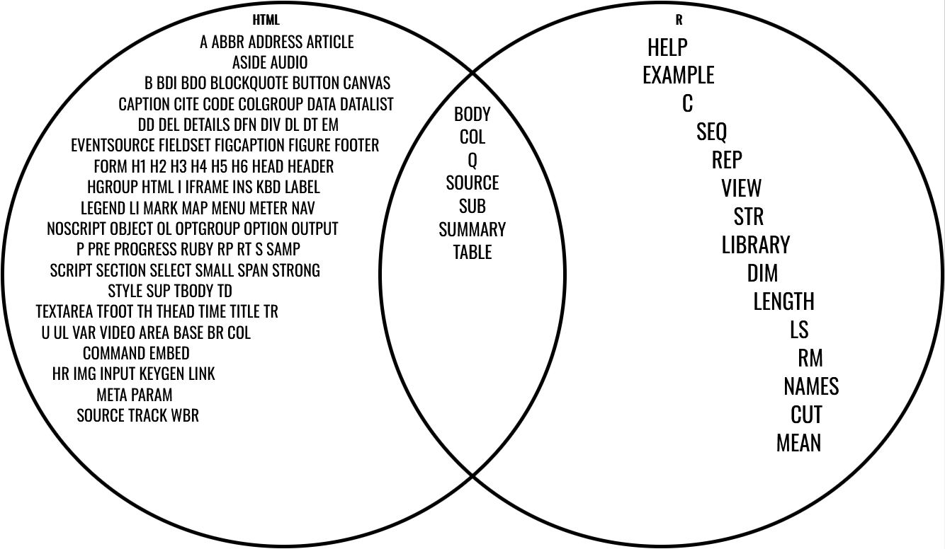
- Solution: first a
list(), then an “environment”
Creating a list makes translation work
#> <HTML> <p class='mypara'>Some text. <b><i>some bold italic
#> text</i></b></p>Creating an environment makes the UX better
#> <HTML> <body><h1 id='first'>A heading</h1><p>Some text &<b>some
#> bold text.</b></p><img src='myimg.png' width='100' height='100'
#> /></body>Fundamentals of R → LaTeX
We can generate LaTeX syntax from R
- We can do this:
That look like this:\[\sin(\pi) + \mathrm{f}(a)\]
By doing this:
We need to know some LaTeX structure for this exercise
- Simple mathematical equations are written like in R:
x * y, z ^ 5= \(x * y, z^5\) - Special characters start with a
\. For example,\pi= \(\pi\) - Complicated functions look like
\name{arg1}{arg2}. For example, fractions are\frac{a}{b}= \(\frac{a}{b}\) - Mathematics functions need to be written like
\textrm{f}(a * b)= \(\textrm{f}(a*b)\)
How to R → LaTeX
Follow a macro-micro procedure to create LaTeX DSL
Start with infrastructure (
to_math()) and experiment until cover every use case.Four stages:
Convert known symbols:
pi→\piLeave other symbols unchanged:
x→x,y→yConvert known functions to their special forms:
sqrt(frac(a, b))→\sqrt{\frac{a}{b}}Wrap unknown functions with
\textrm:f(a)→\textrm{f}(a)
Our LaTeX DSL will be different than our HTML DSL
- Evaluation environment no longer constant
- Has to vary depending on input
- Necessary to handle unknown symbols & functions
- Never evaluate in argument environment
- We translate every function to a LaTeX expression
- User must explicitly
!!in order to evaluate normally
We need to create an execution environment: to_math()
# Execution environment
to_math <- function(x) {
  expr <- enexpr(x) # Capture expression (intended LaTeX)
  out <- eval_bare(expr, latex_env(expr)) # Evaluate in a specific environment for this expression

  latex(out)
}

# Class generator
latex <- function(x) structure(x, class = "advr_latex")

# Dispatch
print.advr_latex <- function(x) {
  cat("<LATEX> ", x, "\n", sep = "")
}
latex_env() is going to be created later. It depends on the expression.
R → LaTeX: translating known symbols
We can quickly create an environment with all the Greek letters
greek <- c(
  "alpha",
  "theta",
  "tau",
  "beta",
  "vartheta",
  "pi",
  "upsilon",
  "gamma",
  "varpi",
  "phi",
  "delta",
  "kappa",
  "rho",
  "varphi",
  "epsilon",
  "lambda",
  "varrho",
  "chi",
  "varepsilon",
  "mu",
  "sigma",
  "psi",
  "zeta",
  "nu",
  "varsigma",
  "omega",
  "eta",
  "xi",
  "Gamma",
  "Lambda",
  "Sigma",
  "Psi",
  "Delta",
  "Xi",
  "Upsilon",
  "Omega",
  "Theta",
  "Pi",
  "Phi"
)
greek_list <- set_names(paste0("\\", greek), greek)
greek_env <- as_environment(greek_list)
Our environment for known symbols works
R → LaTeX: translating unknown symbols
We can capture the unknown symbols from the expression
Leave non-Greek symbols as-is, but we don´t know what symbols are going to be used.
#> [1] "x" "y" "a" "b" "c"Utility functions from section 18.5…
expr_type <- function(x) {
  if (rlang::is_syntactic_literal(x)) {
    "constant"
  } else if (is.symbol(x)) {
    "symbol"
  } else if (is.call(x)) {
    "call"
  } else if (is.pairlist(x)) {
    "pairlist"
  } else {
    typeof(x)
  }
}
flat_map_chr <- function(.x, .f, ...) {
  purrr::flatten_chr(purrr::map(.x, .f, ...))
}
switch_expr <- function(x, ...) {
  switch(
    expr_type(x),
    ...,
    stop("Don't know how to handle type ", typeof(x), call. = FALSE)
  )
}
We can build the environment based on the list of the unknown symbols
We can integrate the known and unknown symbols environments
Our environment for all symbols works
R → LaTeX: translating known functions
We can base our translation on simple helpers
#> function (e1)
#> paste0("\\sqrt{", e1, "}")#> function (e1, e2)
#> paste0(e1, "+", e2)We can build the environment for functions with some common examples
# Binary operators
f_env <- child_env(
  .parent = empty_env(),
  `+` = binary_op(" + "),
  `-` = binary_op(" - "),
  `*` = binary_op(" * "),
  `/` = binary_op(" / "),
  `^` = binary_op("^"),
  `[` = binary_op("_"),

  # Grouping
  `{` = unary_op("\\left{ ", " \\right}"),
  `(` = unary_op("\\left( ", " \\right)"),
  paste = paste,

  # Other math functions
  sqrt = unary_op("\\sqrt{", "}"),
  sin = unary_op("\\sin(", ")"),
  log = unary_op("\\log(", ")"),
  abs = unary_op("\\left| ", "\\right| "),
  frac = function(a, b) {
    paste0("\\frac{", a, "}{", b, "}")
  },

  # Labelling
  hat = unary_op("\\hat{", "}"),
  tilde = unary_op("\\tilde{", "}")
)
We can integrate this new environment to the symbols environment
Our integrated symbol and known functions environment works
R → LaTeX: translating unknown functions
We create a list of unknown functions based on the expression
#> [1] "f" "+" "d"We can use a function factory for creating unknown functions
#> function (...)
#> {
#>     contents <- paste(..., collapse = ", ")
#>     paste0("\\mathrm{foo}(", contents, ")")
#> }
#> <environment: 0x0000025275b4bc10>
We can integrate the unknown function environment
latex_env <- function(expr) {
  calls <- all_calls(expr)
  call_list <- map(set_names(calls), unknown_op)
  call_env <- as_environment(call_list)

  # Known functions
  f_env <- env_clone(f_env, call_env)

  # Default symbols
  names <- all_names(expr)
  symbol_env <- as_environment(set_names(names), parent = f_env)

  # Known symbols
  greek_env <- env_clone(greek_env, parent = symbol_env)
  greek_env
}
Our final environment and the full translation works!
Synthesis
R can translate to HTML via a micro-macro procedure
Creating an S3 for translation and automatic escaping
Creating a tag function structure
Creating a function factory for tags
Creating an execution environment:
with_html()
R can translate to LaTeX via a macro-micro procedure
Build an interface that contains a dynamic environment
Creating and environment of known symbols by declaring them
Creating and environment of unknown symbols by walking the AST of the expression
Creating and environment of known functions by declaring the most common ones
Creating and environment of unknown functions by walking the AST and using a function factory
Integrating all the environment in the dynamic environment contained in the
to_math()interface
Final remarks
This chapter integrates core advanced R concepts
- Code as data
- S3 classes and method dispatch
- Environments and scoping
- Dynamic function generation
Takeaway: R enables languages inside the language
- Translation comes naturally from how R is designed
- Creating small domain-specific languages in R is normal and expected, not a trick
- Advanced R shows how to build them in a clear, safe, and maintainable way